
Abstract
SUMMARY: CT perfusion (CTP) is a functional imaging technique that provides important information about capillary-level hemodynamics of the brain parenchyma and is a natural complement to the strengths of unenhanced CT and CT angiography in the evaluation of acute stroke, vasospasm, and other neurovascular disorders. CTP is critical in determining the extent of irreversibly infarcted brain tissue (infarct “core”) and the severely ischemic but potentially salvageable tissue (“penumbra”). This is achieved by generating parametric maps of cerebral blood flow, cerebral blood volume, and mean transit time.
Part 1 of this review establishes the clinical context of CT perfusion (CTP). Next, a discussion follows on CTP map construction by using the maximal slope method and the 2 main deconvolution techniques, Fourier transformation (FT) and singular value decomposition (the latter being the most commonly used numeric method in CTP). Part 2 discusses the pearls and pitfalls of CTP map acquisition, postprocessing, and image interpretation. Issues including radiation dose−reduction strategies, methods of correcting arterial input function (AIF) delay, the effect of laterality of AIF choice, vascular pixel elimination, the importance of correct cerebral blood flow (CBF) and cerebral blood volume (CBV) threshold selection, and the selection of appropriate perfusion parameters for correct estimation of penumbra are addressed. The review highlights the need for validation and standardization of important CTP parameters to improve patient outcomes and to design future randomized clinical trials that will provide evidence for the importance of the core/penumbra “mismatch” in patient triage for recanalization therapies beyond the current 3-hour therapeutic window for intravenous thrombolysis.
Clinical Context of CTP
The management of acute ischemic stroke remains challenging because there is a limited time window in which diagnosis must be made and therapy administered. Intravenous tissue plasminogen activator (tPA), to be used within 3 hours of stroke onset based on the 1995 National Institute of Neurological Disorders and Stroke trial, and the Mechanical Embolus Removal in Cerebral Ischemia clot retrieval device, to be used within 9 hours of stroke onset, are the only treatments currently approved by the US Food and Drug Administration for acute stroke.1–8 The only imaging technique currently required before intravenous tPA administration is an unenhanced head CT, used to exclude intracranial hemorrhage (an absolute contraindication) and infarct size greater than one third of the middle cerebral artery (MCA) territory (a relative contraindication and predictor of increased hemorrhagic risk following tPA administration).9,10 The strict 3-hour therapeutic window from symptom onset, delays in transportation and triage, and the multiple contraindications to tPA administration, however, all limit the use of intravenous tPA to typically 3%–5% of patients admitted with ischemic stroke.11
There has been increasing interest in advanced CT and MR imaging techniques to extend the traditional anatomic applications of imaging and offer additional insights into the pathophysiology of acute stroke. A wider time-to-treatment window might be achieved in patients who demonstrate a “mismatch” in the size of the ischemic “core” of irreversibly infarcted tissue and hypoperfused “penumbra” (the severely ischemic but potentially salvageable tissue).12–14 There is increasing evidence that core/penumbra mismatch in some patients may persist up to 12 or even 24 hours from the ischemic insult.15,16 Hence, the judicious use of intravenous tPA and endovascular therapy beyond 6–9 hours, by using advanced imaging for patient selection, is currently under intense study.
Acute stroke imaging addresses 4 critical questions17:
Is there hemorrhage?
Is there intravascular thrombus that can be targeted for thrombolysis?
Is there a core of critically ischemic irreversibly infarcted tissue?
Is there a penumbra of severely ischemic but potentially salvageable tissue?
CTP addresses the last 2 questions, after unenhanced CT and CT angiography (CTA) have each addressed the first and the second questions, respectively. The application of CTP was first proposed as early as 1980 by Axel18; however, the CT acquisition and postprocessing systems available at that time were too slow to make CTP a practical reality.
Cerebral perfusion refers to tissue (capillary)-level blood flow. Brain-tissue flow can be described by several parameters, including CBF, CBV, and mean transit time (MTT) (Fig 1). CBV is defined as the total volume of flowing blood in a given volume in the brain, with units of milliliters of blood per 100 g of brain tissue. CBF is defined as the volume of blood moving through a given volume of brain per unit time, with units of milliliters of blood per 100 g of brain tissue per minute. MTT is defined as the average transit time of blood through a given brain region, measured in seconds. “Core” is typically operationally defined as the CBV lesion volume, and “penumbra,” as the MTT or CBF lesion volume.17 “Mismatch” is typically defined, therefore, as the difference between these.
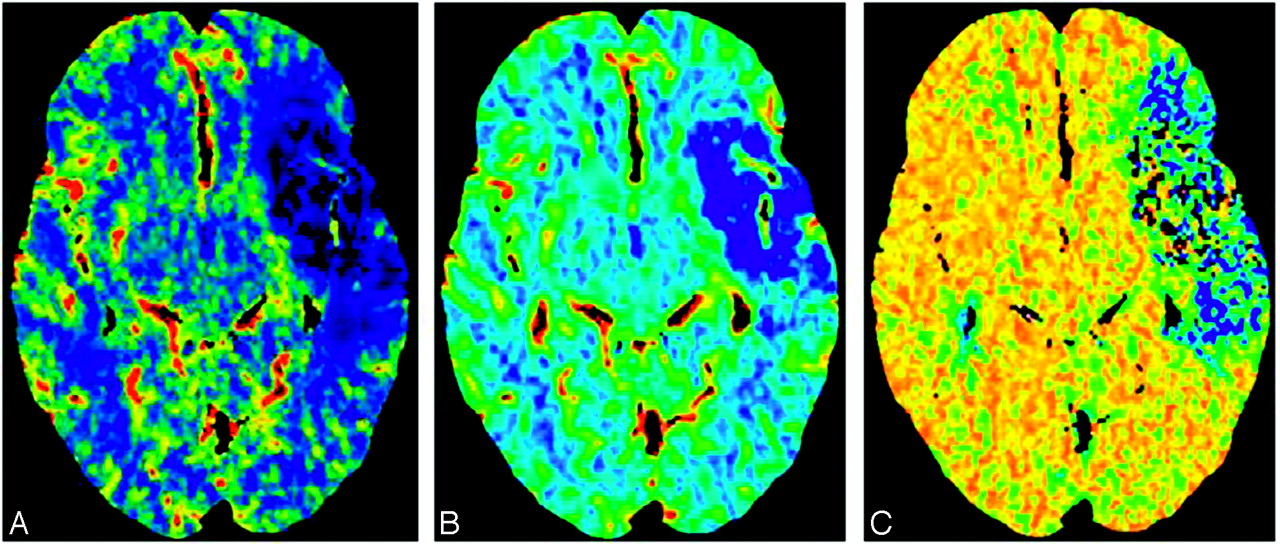
CT perfusion images obtained in a patient with acute ischemic stroke demonstrate a large perfusion defect in the left MCA distribution, with minimal CBV/MTT or CBF mismatch. A, CBF. B, CBV. C, MTT.
The list of completed and ongoing trials by using core/penumbra mismatch as a selection criterion for treatment is long and illustrates the increasingly important role of advanced imaging in acute stroke management. These trials use predefined threshold values for core and penumbra to select patients who can potentially benefit from recanalization. Completed trials include Desmoteplase in Acute Ischemic Stroke (DIAS),12 Dose Escalation of Desmoteplase for Acute Ischemic Stroke (DEDAS),19 Diffusion and Perfusion Imaging Evaluation for Understanding Stroke Evolution (DEFUSE),20 the German Multicenter Trial,21 and Echoplanar Imaging Thrombolysis Evaluation Trial (EPITHET)22; continuing trials include MR and Recanalization of Stroke Clots by using Embolectomy (MR RESCUE).23 CT perfusion can also be applied with nonrecanalization-based neuroprotective therapies for acute stroke.
In present clinical practice, CTP can be used to identify patients with MCA occlusion and core/penumbra mismatch for induced hypertension therapy with phenylephrine (Neosynephrine), even beyond the thrombolysis window.24 High-flow oxygen therapy (hyperbaric or normobaric) is another promising neuroprotective strategy for which patient selection with mismatch imaging may play a role.25,26 Patients in intensive care units who have undergone cardiac surgery might also benefit from CTP; a recent study reported greater sensitivity in detecting and mapping acute ischemic stroke in these patients in whom conventional imaging findings were inconsistent with the severity of clinical condition.27
Secondary cerebral infarction due to subarachnoid hemorrhage (SAH)−related vasospasm is the most significant cause of mortality and morbidity following aneurysm rupture.28 Transcranial Doppler sonography, CTA, and cerebral angiography can all detect angiographic spasm, the visually apparent reduction in vessel caliber. They cannot, however, detect clinical spasm (the syndrome of confusion and decreased level of consciousness resulting from decreased blood flow to the brain). CTP is more sensitive in detecting clinically relevant spasm, measured as a decrease in CBF and delay in MTT,29 than the methods used for angiographic spasm.30 Several studies have demonstrated that CTP is a sensitive and early predictor of secondary cerebral infarction in both patients and animal models with SAH-related clinical spasm.28,30–32
CTP Theory and Modeling
Comparison with MR Perfusion-Weighted Imaging
CTP imaging techniques are relatively new compared with MR imaging−based methods; their clinical applications are, therefore, less thoroughly reported in the literature.33–35 Despite this, because the general principles underlying the computation of perfusion parameters such as CBF, CBV, and MTT are the same for both MR imaging and CT, the overall clinical applicability of perfusion imaging by using either of these techniques is similar. Differences in technique create several important distinctions, however, summarized in Table 1. The most important advantage of CTP is the linear relationship between contrast concentration and attenuation in CT, which facilitates quantitative (versus relative) measurement of CBF and CBV. MR perfusion imaging (MRP) relies on the indirect T2* effect induced in the tissue by gadolinium; the T2* effect itself is not linearly related to the gadolinium concentration, making absolute measurement of CBF and CBV difficult. One disadvantage of CTP is, until recently, the relatively limited coverage, whereas MRP is capable of covering the whole brain during a single bolus injection. For making stroke-related treatment decisions, CTP coverage must be sufficient to scan the entire ischemic territory at risk of infarction.36 A second disadvantage of using CT rather than MR imaging for stroke assessment is the decreased sensitivity for detection of cerebral microbleeds compared with gradient-echo sequences. Microbleeds detected on T2*-weighted MR imaging, however, have been shown not to be a contraindication to thrombolysis.37
Comparison of CTP with MRP imaging
CBV Calculations
The dynamic first-pass approach to CTP measurement involves the intravenous administration of an intravascular contrast agent, which is tracked with serial imaging during its first circulation through the brain tissue capillary bed. The main assumption of dynamic first-pass contrast-enhanced CTP models is that the perfusion tracer is not diffusible, neither metabolized nor absorbed by the tissue through which it traverses. This is certainly the case in a healthy human brain; however, breakdown of the blood-brain barrier (BBB) in infection, inflammation, or tumor adds an additional level of complexity. When extensive BBB breakdown exists, leakage of contrast material into the extravascular space results in overestimation of CT CBV.38
The determination of cerebral perfusion by using CTP is based on examining the relationships between the arterial, tissue, and the venous enhancement. More specifically, tracer kinetic theory states that if one knows the input and the output of a tracer from a voxel, one can determine the volume of distribution (ie, fractional vascular volume) and the clearance rate (ie, flow per unit tissue volume).18,39,40 The fractional vascular volume, f, is defined by the following equation:  1) where Vvasc, Vinterstitium, and Vcells are the volumes occupied by the vascular space, interstitium, and cells, respectively. If the chosen region of interest is devoid of major blood vessels, the measured change in the CT number will reflect the tissue blood pool. The contrast concentration in the tissue, Ctissue, which is measured by the CT scanner, is smaller than the intravascular concentration, Cvasc, by the fraction f,
  2)
2)
The total amount of contrast material delivered to the tissue via the arteries is the product of the CBF times the integral of the arterial concentration, Cartery(t). According to the conservation-of-mass principle, this total amount must be equal to the amount leaving the tissue, that is, the product of CBF with the integral of Cvasc(t).18 Hence,  3)
3)
From equations 2 and 3, it follows that  4)
4)
CBV can be calculated from equation 4 if one takes into account the brain tissue attenuation, ρ, and a correction factor, CH, to adjust the difference between arterial and capillary hematocrit.35,41 In vivo experiments in the 1970s demonstrated the markedly lower hematocrit in capillaries compared with arterial hematocrit42–44; hence, the introduction of the CH is required for the quantification of CBV as follows:  5)
5)
Theoretic modeling has suggested that the source images from a CTA acquisition (CTA-SI) are predominantly blood-volume− rather than blood-flow−weighted, assuming that a steady state of arterial and tissue contrast has been achieved during scan acquisition.18,35,45 Coregistration and subtraction of the unenhanced head CT images from the CTA-SI should, therefore, result in quantitative CBV-weighted maps. This is appealing in clinical practice because CTA-SI subtraction maps, unlike first-pass CTP maps, can provide whole-brain coverage. The change in attenuation due to iodine administration is directly proportional to its concentration; thus, the ratio of the change in Hounsfield units (HU) in brain tissue (ΔHUtissue) and arterial blood (ΔHUartery) can be used in practice to estimate CBV according to the relationship of equation 5 (Fig 2). Specifically, CBV can be expressed in milliliters per 100 g of tissue as follows:  6) where Vvoxel is voxel volume and N is the calculated number of voxels in 100 g of tissue.45

CTA source images acquired during a steady state of contrast concentration for both the arterial and tissue−time-attenuation curves (ΔT) are predominantly blood-volume− rather than blood-flow−weighted. The change in attenuation due to iodine administration is directly proportional to its concentration. CBV equals the ratio of the areas under the 2 curves, Ctissue and Carterial, respectively. This can be approximated as the ratio of the HUtissue/HUarterial when the 2 curves approach steady state.
Although a relative steady state of tissue arterial contrast could be assumed with the multidetector row CT (MDCT) injection protocols used in the 1990s and early 2000s, in which low contrast-injection rates were applied with relatively long prep delay times (typically 3 mL/s, and >25 seconds),45 this steady-state assumption no longer holds in this era of newer faster MDCT CTA protocols, such as those used in 64-section scanners, in which injection rates ≤7 mL/s and short prep delay times of 15–20 seconds change the temporal shape of the time-attenuation infusion curve, eliminating a near steady state during the timing of the CTA-SI acquisition. Hence, with the current implementation of CTA protocols on faster state-of-the-art MDCT scanners, the CTA-SI maps have become more flow-weighted than volume-weighted.
Mathematic Models for CBF and MTT Calculation
The 2 major mathematic approaches involved in calculating CBF and MTT are the deconvolution- and nondeconvolution-based methods. Deconvolution techniques are technically more demanding and involve more complicated and time-consuming processing, whereas nondeconvolution techniques are more straightforward but depend on simplified assumptions regarding the underlying vascular architecture. As a result, the interpretation of studies based on nondeconvolution methods may be less reliable in some situations, though this has not been fully clinically validated.
Nondeconvolution-Based Models
Like deconvolution methods, nondeconvolution methods are based on the application of the Fick principle of conservation of mass to a given region of interest within the brain parenchyma (Fig 3). The accumulated mass of contrast, Q(T), in a voxel of brain tissue during a time period corresponding to the complete wash in and wash out of contrast during a bolus injection (with a saline “chaser”) is equal to the product of CBF and the time integral of the arteriovenous difference in contrast concentration:  7)
7)

Fick Principle.
One immediate simplification that would make solving this equation less computationally intensive is to assume that during the above time period, the venous concentration is zero (ie, no contrast has yet reached the venous side of the circulation, the “no venous outflow” assumption). This assumption is valid only when T is <4–6 seconds, the minimum transit time of blood through the brain. Under this assumption, equation 7 can be simplified as follows:  8)
8)
This is known as the Mullani-Gould formulation or single-compartment formulation.46
When rewriting equation 8 into its derivative form for easier calculation of CBF,  9) it follows that the rate of contrast accumulation will peak when the arterial concentration is maximal:
  10)
10)
Hence, CBF is the ratio of the maximum slope of Q(t) to the maximum arterial concentration. This is analogous to a differentiation with respect to time of the Mullani-Gould formulation and is called the “maximum slope method”. The principal advantage of the maximum slope method is the simplicity and hence speed of calculation of the perfusion values. A very high rate of contrast agent injection, however, is required—typically at least 10 mL/s—to satisfy the no-venous-outflow assumption.47,48 These rates cannot be routinely achieved in clinical practice. The no-venous-outflow assumption is clearly an oversimplification, and this method yields relative, rather than absolute, perfusion measurements, making interpatient or interinstitutional comparison of results difficult.
Deconvolution-Based Models
Considering a bolus of contrast tracer material injected into a tissue voxel of interest, we can define the concentration Ctissue(t) of tracer in the tissue in terms of 2 functions:
) Residue function, R(t): a fraction of tracer is still present in the voxel of interest at time t following an ideal instantaneous unit bolus injection. R(t) is unitless and is equal to 1 at t = 0 49;
) AIF, Cartery(t): concentration of tracer in the feeding vessel to the voxel of interest at time t.
Calculation of CBF requires measurement of the temporal shape of both the arterial input and the tissue−time-attenuation curves.40,50 The true input into the tissue voxel of interest cannot be measured directly; in practice, the AIF is estimated from a major artery (eg, the MCA or the “top” of the internal carotid artery), with the assumption that this represents the exact input to the tissue of interest. Any delay or dispersion of the bolus introduced during its passage from the artery used for AIF estimation to the tissue of interest will introduce errors in quantification of CBF.51,52
The observed tissue−time-attenuation curve represents a combination of the effects of the AIF and the inherent tissue properties. Thus, to fit the model, the effects of the AIF on the tissue concentration curve must be removed by using a mathematic process known as “deconvolution” to derive R(t), which is dependent only on the hemodynamic properties of the voxel under consideration. R(t) demonstrates an abrupt (indeed instantaneous) rise, a plateau of duration equal to the minimum transit time through the tissue of interest and then decay toward baseline. It was shown by Meier and Zieler53 that the tissue concentration curve can be represented as the CBF multiplied by AIF convolved with R(t):  11) where “⊗” is the convolution operator, ρ is the brain tissue attenuation, and CH is the correction factor for the capillary hematocrit levels. Ctissue and AIF are measured directly from the time-attenuation curve from the cine CTP source images, and the problem then becomes the calculation of CBF and R(t). Several methods to “deconvolve” equation 11 and hence solve for CBF and R(t) have been proposed and are divided into 2 main categories. With parametric methods, a specific analytic expression for R(t) is assumed. Assuming a specific shape for R(t) imposes assumptions on the inherent tissue properties that cannot be known a priori with sufficient precision.50,54,55 Due to this limitation, the most commonly used methods have become the nonparametric ones, which do not assume a shape for R(t).
Deconvolution of equation 11 is unstable, in the sense that it frequently yields nonphysiologic oscillations (ie, noise) in the computation of the solution for R(t). The nonparametric approach can be further subdivided in 2 categories, which differ in the way in which they deal with noise resulting from the instability of deconvolution.56 In the first, the transform approach, the convolution theorem of the FT is used to deconvolve equation 11. The theorem states that the FT of the convolution of 2 time-domain functions is equivalent to the multiplication of their respective FTs.50,57,58 With the convolution theorem, equation 11 can be rewritten as  12) where ℑ is the Fourier transform. R(t) and CBF can thus be determined by taking the inverse FT of the ratios of the 2 transforms of the sampled AIF(t) and Ctissue(t). However, this approach is very sensitive to noise, as demonstrated by Ostergaard et al.55
The second approach, the more commonly applied singular value decomposition (SVD), is an algebraic reformulation of the convolution integrals of equation 11 rewritten as  13) where t1, t2,…tN are equally spaced time points and AIF(t) and Ctissue(t) are measured. Equation 13 can be rewritten in shorthand matrix-vector notation:
  14) where b and c are vectors whose elements are R(ti) and Ctissue(ti), respectively, and A is the convolution matrix in equation 13. It can be shown that the least squares solution for b is given by (AT · A)−1 · AT, where AT is the transpose of the convolution matrix and (AT · A)−1 is the inverse of the symmetric matrix AT · A.59 SVD decomposes A into a product of matrices, such that (AT · A)−1 can be found easily and the solution for b can be written as a sum of terms weighted by the reciprocal of the singular values of A.60 By truncating small singular values in the sum for the solution vector b, oscillations from noise in the both AIF(t) and Ctissue(t) are avoided.
SVD has yielded the most robust results from all the deconvolution methods used to map CBF55 and has gained widespread acceptance. The creation of accurate quantitative maps of CBF, CBV, and MTT by using deconvolution methods has been validated in a number of studies.61–67 Once CBF and CBV are known, MTT can be calculated from the ratio of CBV and CBF, by using the central volume theorem.53,68
Potential pitfalls in the computation of CBF by using deconvolution methods include patient motion and partial volume averaging, which can cause underestimation of the AIF(t). Image-coregistration software to correct for patient motion and careful choice of regions of interest for the AIF can minimize these pitfalls.
Commercial software suppliers use different mathematic methods. In the past, some have incorporated the maximum slope method, though new versions are frequently released and the reader is advised to check for the most up-to-date software from each vendor. Others have typically used deconvolution techniques, which, though theoretically superior to nondeconvolution methods—as has already and will again to be noted—the full clinical implication of using has yet to be established and standardized by the stroke imaging community.
Validation of CTP
CBF quantification with CTP has been preliminarily tested in animals and humans. In animals, the accepted reference standard method for quantifying CBF is the microsphere technique and, to a lesser extent, postmortem histology. CTP measurements have been validated in healthy animals, animals with experimental ischemic stroke, and animals with implanted tumors.61,62,64,66,69 All studies reported very good correlation between CTP and the reference-standard methods (Table 2). In humans, CTP has been validated with positron-emission tomography and xenon-enhanced CT in healthy subjects, patients with acute stroke, and patients with chronic cerebrovascular disease. Some of these studies are summarized in Table 2. Deconvolution-based CTP studies by Wintermark et al67 and Kudo et al70 gave slopes within 13% of unity, whereas the difference from unity was 20%–60% for the maximum slope technique used by Sase et al (2005).71 These results once again suggest a superior accuracy of deconvolution techniques compared with maximum slope−based methods.
Animal and human studies validating CTP
References
- Copyright © American Society of Neuroradiology
In this issue


Jump to section
Related Articles
Cited By...
- Reducing False-Positives in CT Perfusion Infarct Core Segmentation Using Contralateral Local Normalization
- Detecting CTP Truncation Artifacts in Acute Stroke Imaging from the Arterial Input and the Vascular Output Functions
- Defining Ischemic Core in Acute Ischemic Stroke Using CT Perfusion: A Multiparametric Bayesian-Based Model
- Whole-brain Volume Perfusion Computed Tomography: Acquisition Techniques and Radiation Dose
- Admission CT perfusion may overestimate initial infarct core: the ghost infarct core concept
- Comparison of Perfusion CT Software to Predict the Final Infarct Volume After Thrombectomy
- Occult Anterograde Flow Is an Under-Recognized but Crucial Predictor of Early Recanalization With Intravenous Tissue-Type Plasminogen Activator
- Whole-Brain Adaptive 70-kVp Perfusion Imaging with Variable and Extended Sampling Improves Quality and Consistency While Reducing Dose
- A Novel Technique for the Measurement of CBF and CBV with Robot-Arm-Mounted Flat Panel CT in a Large-Animal Model
- Comparison of Computed Tomographic and Magnetic Resonance Perfusion Measurements in Acute Ischemic Stroke: Back-to-Back Quantitative Analysis
- Pretreatment Advanced Imaging in Patients with Stroke Treated with IV Thrombolysis: Evaluation of a Multihospital Data Base
- Can Iterative Reconstruction Improve Imaging Quality for Lower Radiation CT Perfusion? Initial Experience
- Differences in CT Perfusion Summary Maps for Patients with Acute Ischemic Stroke Generated by 2 Software Packages
- Application of acute stroke imaging: Selecting patients for revascularization therapy
- CT Angiographic Source Images: Flow- or Volume-Weighted?
- Evaluation of CT Perfusion in the Setting of Cerebral Ischemia: Patterns and Pitfalls
- FDA Investigates the Safety of Brain Perfusion CT
- Theoretic Basis and Technical Implementations of CT Perfusion in Acute Ischemic Stroke, Part 2: Technical Implementations