
Abstract
BACKGROUND AND PURPOSE: The 45° oblique (Pöschl) plane allows reliable depiction of the vestibular aqueduct, with virtually its entire length often visible on 1 CT image. We measured its midpoint width in this plane, aiming to determine normal measurement values based on this plane.
MATERIALS AND METHODS: We retrospectively evaluated temporal bone CT studies of 96 pediatric patients without sensorineural hearing loss. Midvestibular aqueduct widths were measured in the 45° oblique plane by 2 independent readers by visual assessment (subjective technique). The vestibular aqueducts in 4 human cadaver specimens were also measured in this plane. In addition, there was a specimen that had undergone CT scanning before sectioning, and measurements made on that CT scan and on the histologic section were compared. Measurements from the 96 patients' CT images were then repeated by using findings derived from the radiologic-histologic comparison (objective technique).
RESULTS: All vestibular aqueducts were clearly identifiable on 45° oblique-plane CT images. The mean for subjective measurement was 0.526 ± 0.08 mm (range, 0.337–0.947 mm). The 97.5th percentile value was 0.702 mm. The mean for objective measurement was 0.537 ± 0.077 mm (range, 0.331–0.922 mm). The 97.5th percentile value was 0.717 mm.
CONCLUSIONS: Measurements of the vestibular aqueduct can be performed reliably and accurately in the 45° oblique plane. The mean midpoint width was 0.5 mm, with a range of 0.3–0.9 mm. These may be considered normal measurement values for the vestibular aqueduct midpoint width when measured in the 45° oblique plane.
ABBREVIATIONS:
- LVA
- large vestibular aqueduct
- OPA
- optimal percentage attenuation
Valvassori and Clemis1,2 reported in 1978 that the vestibular aqueduct may be considered enlarged when its width at midpoint measures >1.5 mm on hypocycloidal polytomography. CT has since replaced tomography as the technique of choice for temporal bone evaluation. In 2007, Boston et al3 proposed a new definition of an enlarged vestibular aqueduct based on axial CT studies. The criteria they established, referred to as the Cincinnati criteria, defined large vestibular aqueduct (LVA) as a vestibular aqueduct with width of ≥2 mm at the operculum and/or ≥1 mm at the midpoint as measured on axial images.
Current scanners allow CT source images to be reformatted in any plane with near-identical spatial resolution.4,5 This feature is used in temporal bone imaging for optimizing visualization of various anatomic structures. In particular, the 45° oblique (Pöschl) plane has been shown to depict the vestibular aqueduct more reliably than the axial plane because this plane is parallel to the longitudinal axis of the vestibular aqueduct, and this plane allows depiction of virtually the entire length of this structure.6,7 Evaluation of the vestibular aqueduct in this plane allows accurate identification of its midpoint and determination of its true cross-sectional width without overestimation related to obliquity (Fig 1).
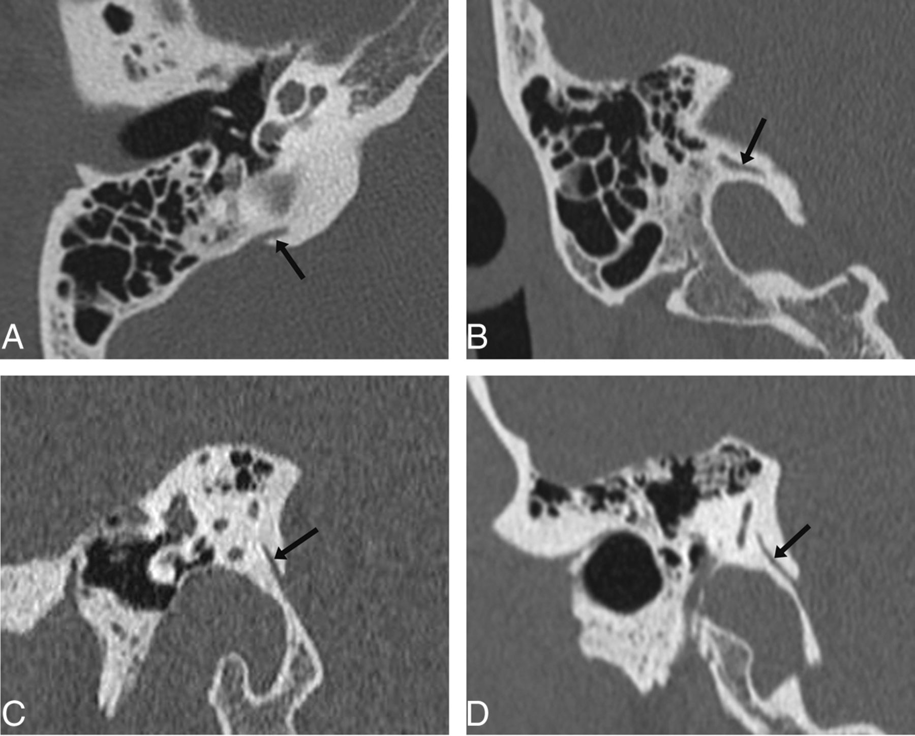
The vestibular aqueduct as seen on axial (A), coronal (B), sagittal (C), and the 45° oblique (Pöschl) (D) planes (arrows). It can be seen along its entire longitudinal length on the 45° oblique plane, but only partially on the other planes. It also appears wider on the axial, coronal, and sagittal planes, due to the oblique orientation of its cross-section relative to these planes, which may lead to overestimation of its width when measurement is made in these planes.
In this study, we aimed to determine normal measurements for the vestibular aqueduct midpoint width based on the 45° oblique plane.
Materials and Methods
Part 1: CT Measurements, with Caliper Placement Based on Visual Assessment of Bony Margins (Subjective Technique)
Subjects.
Temporal bone CT studies of 96 children (192 vestibular aqueducts) referred from the pediatric otolaryngology service were reviewed retrospectively in accordance with guidelines from the Massachusetts Eye and Ear Infirmary institutional review board. Patients with sensorineural hearing loss were excluded from the study.
CT Scanning and Processing.
All patients underwent dedicated temporal bone CT without intravenous contrast on a 40-section multidetector CT scanner (Somatom Sensation 40; Siemens, Erlangen, Germany). Images were obtained with 0.6-mm collimation, 0.6-mm thickness, and a 0.2-mm increment at 320 mAs and 120 kV(peak). Data were reconstructed separately for each temporal bone in the axial plane by using a bone algorithm; this was performed routinely in all cases by the CT technologist. However, 45° oblique reformations were not routinely produced in all cases. Thus, for this study, the dataset from each case was transferred to a workstation for postprocessing by using a commercially available 3D reformatting software (Voxar 3D; Barco, Edinburgh, Scotland). On this software, images in the 45° oblique plane were produced for each temporal bone by selecting the plane parallel to the superior semicircular canal and by using that as the landmark image. These reformatted images were then analyzed. The image section demonstrating the entire length of the vestibular aqueduct was selected, enlarged, and exported at full resolution to an open-source software, ImageJ (National Institutes of Health, Bethesda, Maryland), for performing measurements and statistical analyses.
CT Image Evaluation and Measurement: Visual Assessment Technique.
Two neuroradiologists (E.Y.T. and V.M.) independently reviewed the exported images, which were magnified approximately 15 times and viewed at high resolution with a small FOV in bone window settings (width, 4000 HU; level, 700 HU). For each image, the vestibular aqueduct width was measured at the midpoint of the postisthmic segment (Fig 2). Because object edges do not appear absolutely sharp on images, especially when magnified, we paid careful attention to the placement of electronic calipers at the perceived edge of the bony canal of the vestibular aqueduct, aiming to locate the point along the gray zone between white (bone) and dark gray (soft tissue) that best represented the transition from bone to soft-tissue attenuation. Each radiologist measured each vestibular aqueduct twice, with a 1-month time interval between the 2 measurements.

CT image of the vestibular aqueduct in the 45° oblique plane. The midpoint of the vestibular aqueduct is identified, and a line (shown in black) is drawn perpendicular to its wall. The width is measured along this line.
Part 2: Cadaveric Specimen Measurement
Cadaveric Specimen Preparation.
Temporal bones from patients with normal hearing in life were selected from the cadaveric collection at the Otopathology Laboratory at the Massachusetts Eye and Ear Infirmary. All temporal bones were processed in the standard manner for light microscopy,8 including serial sectioning at a thickness of 20 μm and staining of every tenth section by using hematoxylin-eosin. The stained sections were mounted onto glass slides. Only those specimens aligned and sectioned in the plane of the superior semicircular canal could be used, to replicate the 45° oblique plane. This feature limited the number of available specimens to 4.
Cadaveric Specimen Evaluation and Measurement.
Each slide-mounted section that best displayed the entire length of the vestibular aqueduct was reviewed by light microscopy. Measurements were taken at the midpoint of the vestibular aqueduct.
Part 3: Correlation between Measurements Made on Histologic Sections and Measurements Made on CT Images of the Same Cadaveric Specimen
One cadaveric specimen from a patient with normal hearing in life underwent CT scanning before histologic preparation, by using the same CT technique as that for clinical patients. To increase spatial resolution and accuracy, we stained every fifth section through the region of the vestibular aqueduct rather than every tenth. The microtome section that best displayed the entire length of the vestibular aqueduct was paired to the corresponding CT image and reformatted in the 45° oblique plane (Fig 3), and their midpoint widths were measured and compared.
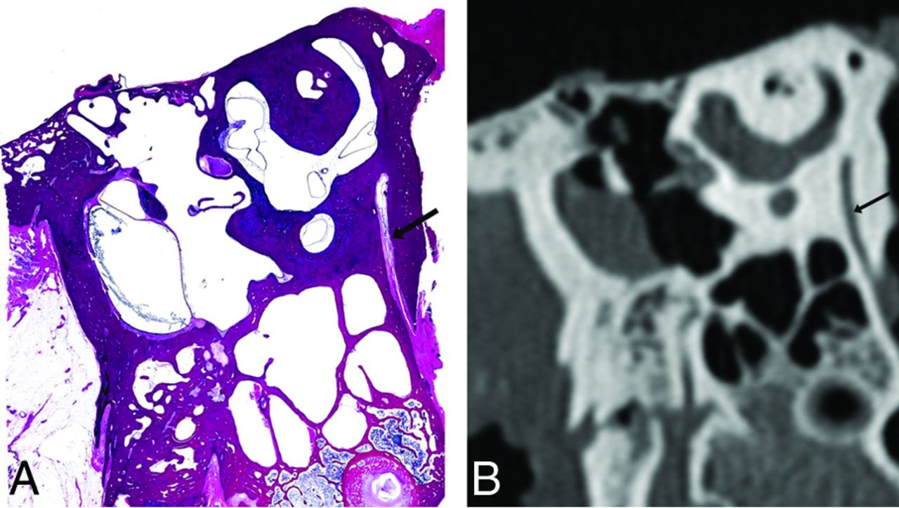
The vestibular aqueduct of a cadaveric temporal bone displayed in the 45° oblique plane (arrow), in a histologically processed microtome section (A) and in a CT image (B).
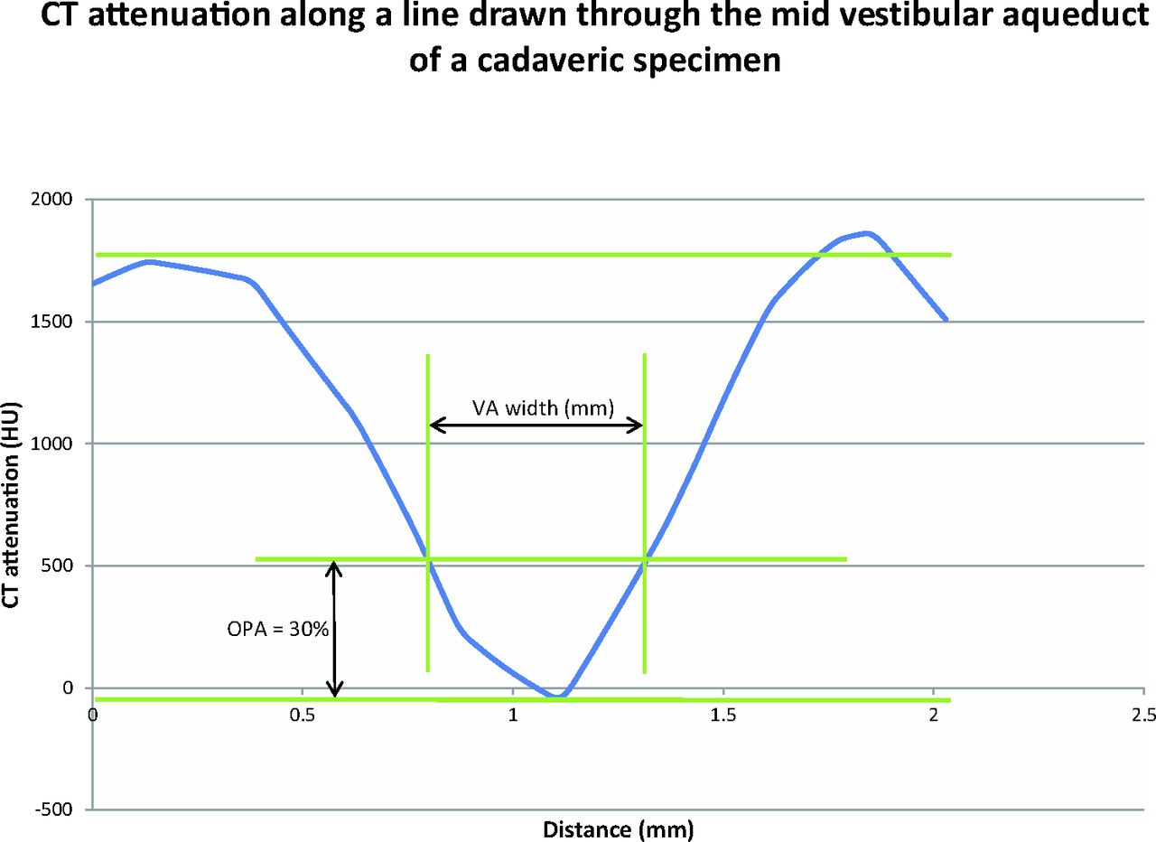
A graph was created by placing calipers on the magnified CT image and recording the CT attenuation (in Hounsfield units) at each pixel along a line drawn through the midpoint of the vestibular aqueduct perpendicular to its wall. The x-axis represented the distance along this line, and the y-axis represented the CT attenuation (Fig 4). This yielded a “CT attenuation curve,” which, instead of being a step function at each bone–soft tissue interface on either end (such as when object edges are absolutely sharp), is a curve. The maximum y-values forming plateaus on either end of the curve (y-max) represent the CT attenuation of bone, and the minimum y-value at the nadir of the curve (y min) represents the CT attenuation in the center of the vestibular aqueduct. For each y-value, the difference between the 2 corresponding x-values (x1 and x2) gives the width of the vestibular aqueduct (x2 − x1, full width). We divided the difference between the maximum and minimum y-values (y-max − y-min) into 10 percentiles. At each percentile, we calculated the corresponding width of the vestibular aqueduct. The percentile at which the vestibular aqueduct width most closely matched the width as measured on the sectioned specimen was noted. This percentile is referred to as the optimal percentage attenuation (OPA) (Fig 4), the point at which placement of electronic calipers on a CT image would lead to a vestibular aqueduct width value that best correlates with the measurement performed on the histologic specimen (best radiologic-histologic correlation).

A graph of the distance along a line drawn through the midpoint of the vestibular aqueduct (x-axis) plotted against CT attenuation in Hounsfield units at each point along this line (y-axis). The optimal percentage attenuation is denoted on the graph. Through radiologic-histologic correlation by using the cadaveric temporal bone specimen, the OPA was found to be 30%.
Part 4: CT Measurements, with Caliper Placement Based on Optimal Percentage Attenuation (Objective Technique)
The CT images from the 96 children that best displayed the vestibular aqueduct and were exported to ImageJ were again reviewed by the 2 neuroradiologists. These images were magnified approximately 15 times and again viewed at high resolution with a small FOV in bone window settings (width, 4000 HU; level, 700 HU). However, instead of placing electronic calipers at the perceived edges by subjective visual assessment, we applied the OPA technique. First, the Hounsfield unit of bone was measured. Then the Hounsfield unit of the desired pixels (HU Desired Pixel) on which to place the calipers was determined by the following equation: [(HU Bone − HU Desired Pixel) / HU Bone] × 100% = OPA. The 2 pixels on either side of the vestibular aqueduct having this Hounsfield unit were selected, and calipers were placed on them for measurement of the vestibular aqueduct width.
Statistical Analysis
Each vestibular aqueduct was measured 5 times (twice for each radiologist using the visual assessment technique, once using the OPA technique).
The measurements made by each radiologist by using the visual assessment technique were analyzed; we calculated the mean, SD, and range for each radiologist (Table 1).
Vestibular aqueduct width obtained using the subjective and objective techniquesa
Pearson correlation coefficients (r) were used to assess the precision of the measurements (Table 2). We calculated them for correlation among the following:
Each radiologist's measurement by using the visual assessment technique and his or her own measurement by using the same technique obtained 1 month later (intraobserver correlation)
One radiologist's measurement using the visual assessment technique and the other radiologist's measurement using the same technique (interobserver correlation)
Each radiologist's measurement using the visual assessment technique (averaged between the 2 measurements obtained 1 month apart) and the measurement obtained by using the OPA technique
The two radiologists' combined measurement (averaged among the 4 values obtained by the 2 radiologists) by using the visual assessment technique and the measurement obtained by using the OPA technique.
Pearson correlation coefficients to determine the precision of various measurements made
Interobserver correlation was obtained by using the first measurement of radiologist A with the second measurement of radiologist B, and the second measurement of radiologist A with the first measurement of radiologist B, to reduce potential bias. Statistical analyses were performed by using SPSS Statistics for Windows (IBM, Armonk, New York).
Results
The 96 patients (51 male and 45 female) had a mean age of 11.0 ± 4.5 years (range, 2–21 years). All vestibular aqueducts were readily identified on the 45° oblique reformations.
For measurements made by using the visual assessment (subjective) technique, the mean midpoint width of the postisthmic segment of the vestibular aqueduct was 0.527 ± 0.08 mm (left side only: 0.524 ± 0.083 mm; right side only: 0.529 ± 0.080 mm). The range was 0.353–0.887 mm. The value at the 95th percentile was 0.666 mm. The value at the 97.5th percentile was 0.702 mm (Table 1).
The optimal percentage attenuation was found to be 30% (Fig 4). In other words, the pixel with the CT attenuation value that is 30% of the difference between the CT attenuation of the center of the vestibular aqueduct and the CT attenuation of the bony margin is the best location for caliper placement on either edge of the vestibular aqueduct that would yield the measurement value closest to that obtained when measuring the actual anatomic structure.
For measurements made by using the OPA technique, the mean midpoint width of the postisthmic segment was 0.537 ± 0.077 mm. The range was 0.331–0.922 mm. The value at the 95th percentile was 0.658 mm. The value at the 97.5th percentile was 0.717 mm (Table 1).
The mean midpoint width of the cadaveric specimens was 0.441 ± 0.134 mm.
Intraobserver, Interobserver, and Intertechnique Reliability
A Pearson correlation coefficient of >0.70 indicates a very strong positive relationship, and a value between 0.40 and 0.69 indicates a strong positive relationship. The measurements made before and after a 1-month interval for the same radiologist (intraobserver reliability) did not demonstrate much variability (r = 0.538 and r = 0.648 for the 2 radiologists). There was also good interobserver correlation (r = 0.506 and r = 0.522). Correlation between measurements made with the 2 techniques showed a strong positive relationship as well (r = 0.566) (Fig 5 and Table 2).
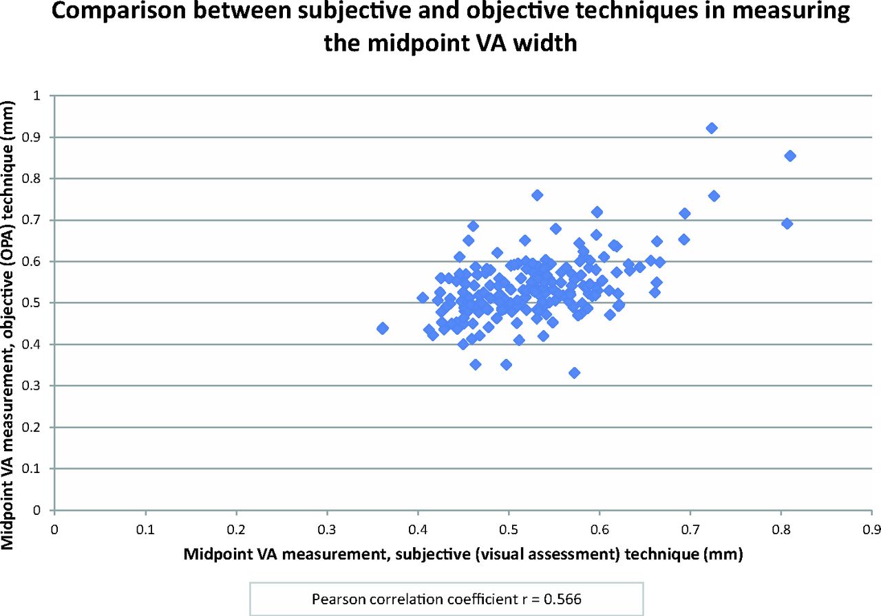
Scatterplot showing comparison between the subjective and objective techniques. Each point denotes the midpoint vestibular aqueduct measurement made by using the subjective (visual assessment) technique (x-axis) plotted against that made by using the objective (modified full width at half maximum/OPA) technique (y-axis). The Pearson correlation coefficient is r = 0.566.
Discussion
CT and MR imaging are important components in the evaluation of congenital sensorineural hearing loss for excluding structural abnormalities.9 Abnormal imaging findings can be seen in 32%–39% of children with sensorineural hearing loss,10 the most common of which is a large vestibular aqueduct. LVA typically has a flared morphology and is often associated with other inner ear malformations,11 including modiolar deficiency with or without incomplete partition type II.12 In 1978, Valvassori and Clemis2 coined the term “large vestibular aqueduct syndrome” to describe children with sensorineural hearing loss, often progressive, with LVA.
The goal of this study was to determine normal measurement values for the normal vestibular aqueduct midpoint width in the 45° oblique plane. This plane was chosen because it allows more reliable and accurate depiction of the vestibular aqueduct along its longitudinal axis compared with the axial plane.6 This follows the basic geometric principle that the optimal planes for displaying a symmetric structure are planes parallel and perpendicular to its main axes of symmetry. Because the vestibular aqueduct is a channel oriented essentially 45° from the sagittal and coronal planes, running from posteroinferior to anterosuperior, the 45° oblique (Pöschl) plane is ideal for displaying the entire length of this structure. In this plane, its midpoint width can be more easily and accurately identified and measured compared with any other plane (eg, axial and coronal). In fact, the 45° oblique plane is the CT counterpart to the transverse pyramidal plane emphasized by Valvassori,1 Valvassori and Clemis,2 Valvassori et al,13 and Becker et al14 as the ideal plane for assessing the vestibular aqueduct tomographically.
The anatomy and development of the vestibular aqueduct have been well-described in the literature.2,15⇓⇓⇓–19 During fetal development, the vestibular aqueduct initially describes a straight course, paralleling the common crus. The aqueduct develops its adult form with the downward pull of the endolymphatic system by the sigmoid sinus and adjacent dura during growth of the posterior fossa. This process results in the originally straight vestibular aqueduct adopting an inverted J shape when viewed in profile. The narrow proximal (superior, anterior, medial) segment (termed “isthmus”) ascends over a short distance, representing the short limb of the J. In our experience, this portion is not well-visualized by CT due to its small size relative to CT voxel size and partial volume effect. The longer distal or postisthmic segment descends toward its external aperture (inferior, posterior, lateral), representing the long limb of the J. This segment is shaped like a thick triangular slab, with the apex at its junction with the isthmus and the broad base at the external aperture.20 The long axis of symmetry runs almost exactly parallel to the 45° oblique plane; in this plane, the vestibular aqueduct can be seen along its entire postisthmic length and demonstrates a fairly uniform width (thickness of the triangular slab) with only minor undulation. On the other hand, the axial, coronal, and sagittal planes pass at varying obliquities through the vestibular aqueduct; measurements made in these planes may therefore result in overestimation of its width. In addition, the ability to view the entire postisthmic segment in the 45° oblique plane allows us to accurately define its midpoint, while this point can only be estimated when in the axial, coronal, and sagittal planes.
While other authors have suggested measuring the vestibular aqueduct at both the midpoint and external aperture, we chose to limit our assessment to the midpoint. Being able to visualize the entire length of the postisthmic segment in the 45° oblique plane allows reliable identification of the midpoint. In this plane, the walls of the normal vestibular aqueduct run parallel to each other and the width is fairly constant; these features allow us to identify and measure the midpoint width with a high degree of certainty and reproducibility. In contrast, the flared configuration of the normal vestibular aqueduct at the external aperture creates difficulty with defining the exact point at which a measurement there should be made, and it is virtually impossible to determine a width perpendicular to the bony margins without a large degree of uncertainty and very limited reproducibility.
Our study shows that the vestibular aqueduct can be accurately measured in the 45° oblique plane on CT images with excellent interobserver and intraobserver reliability. With this method, the normal vestibular aqueduct midpoint width falls within the range of 0.3–0.9 mm. The mean value of 0.5 mm is statistically independent of age or sex. The 97.5th percentile value is 0.7 mm.
One major source of interobserver variation was likely related to the difficulty in determining the edge of the vestibular aqueduct. At low magnification, the edge of the vestibular aqueduct appears fairly distinct; however, at increasing degrees of magnification, it becomes clear that the edge is actually a blur of gray-scale densities. The width of this gray zone is particularly significant relative to the submillimeter size of the vestibular aqueduct. We sought to minimize this edge error by comparing measurements performed by caliper placement using subjective visual assessment with those performed using a modified full width at half maximum technique, which we termed the “optimal percentage attenuation technique.” Given that there is no criterion standard for defining the “true” edge on a pixelated image, we attempted to provide a standard by comparing a midpoint measurement made on a 45° oblique plane CT image of a cadaveric temporal bone with a midpoint measurement made in that same plane on a histologic section of that specimen. Comparison of these 2 measurements helped establish an objective method of CT caliper placement that would yield a measurement that best correlated with the actual anatomic structure. We found that the best correlation occurred when the full width was measured at 30% of the maximum difference in CT attenuation across the vestibular aqueduct (OPA = 30%) (Fig 4).
We repeated the measurements made on the CT images of our patient population by using this modified full width at half maximum/OPA technique, by using the 30% CT attenuation to help us choose the pixels for caliper placement. We found that the results obtained by using this objective technique did not differ significantly from the results obtained by using the subjective technique of visually estimating the perceived edge of the vestibular aqueduct. This finding reassured us that the visual estimation technique is adequate for making measurements on CT images on a practical basis.
One limitation of this study was the small number of histologic specimens available for comparison. Many factors limit their availability, including logistics related to postmortem and histologic processing, incomplete clinical histories and data,8 and the limited number of specimens that had undergone CT scanning before histologic processing to allow radiologic-histologic comparisons (though currently every temporal bone specimen designated for histologic processing at our Otopathology Laboratory undergoes imaging beforehand). In addition, the specimens included were procured specifically to be sectioned in a plane as close as possible to the 45° oblique plane, and preparation time for each specimen was approximately 2 years. Vestibular aqueduct measurements in microdissection specimens have been performed by others and reported in the literature.16,18,21⇓⇓–24 Of these, only Sando and Ikeda24 measured the midpoint width of the vestibular aqueduct. They reported the midvestibular aqueduct measurements in 27 normal temporal bones (28–102 years of age; mean, 66 years) with a mean of 0.48 ± 0.17 mm, similar to the range we obtained from our specimens. Although specimens are subject to various primary and secondary artifacts during their preparation,8 we believe that by using the best available equipment and technique for preparation, we were able to derive important information from even a small number of histologic specimens in terms of the range of measurements to expect and for developing the modified full width at half maximum/OPA technique.
At Massachusetts Eye and Ear Infirmary, we consider vestibular aqueducts measuring 0.8 mm (above the 97.5th percentile value) at midpoint in the 45° oblique plane as borderline to slightly enlarged. Of note, however, there has never been direct correlation between minor enlargement and clinical findings.
Conclusions
The 45° oblique plane allows visualization of the vestibular aqueduct along its longitudinal axis, which, in turn, allows the midpoint and width of the vestibular aqueduct to be readily and accurately identified and measured. We present 2 different measurement techniques in the 45° oblique plane, their corresponding normal range of values, and the results of radiologic-histologic comparison measurements. The mean midpoint width of the vestibular aqueduct was 0.527 ± 0.08 mm when measured by using the subjective visual assessment technique and 0.537 ± 0.077 mm when measured by using the objective 30% optimal percentage attenuation technique. The 95th percentile values were 0.666 and 0.658 mm, respectively, and the 97.5th percentile values were 0.702 and 0.717 mm, respectively. These may be considered normal measurement values of the normal vestibular aqueduct midpoint width when measured in the 45° oblique plane.
Footnotes
Disclosures: Hugh D. Curtin—UNRELATED: Payment for Lectures (including service on Speakers Bureaus): Continuing Medical Education activities (nothing with industry; both paid and unpaid); Royalties: Elsevier (textbook royalties).
Indicates open access to non-subscribers at www.ajnr.org
REFERENCES
- Received October 8, 2015.
- Accepted after revision December 18, 2015.
- © 2016 by American Journal of Neuroradiology


Jump to section
Related Articles
Cited By...
- Does CISS MRI Reliably Depict the Endolymphatic Duct in Children with and without Vestibular Aqueduct Enlargement?
- Retrospective Analysis of the Association of a Small Vestibular Aqueduct with Cochleovestibular Symptoms in a Large, Single-Center Cohort Undergoing CT
- Re-Examining the Cochlea in Branchio-Oto-Renal Syndrome: Genotype-Phenotype Correlation
- Retrospective Review of Midpoint Vestibular Aqueduct Size in the 45{degrees} Oblique (Pöschl) Plane and Correlation with Hearing Loss in Patients with Enlarged Vestibular Aqueduct
- MRI Evaluation of the Normal and Abnormal Endolymphatic Duct in the Pediatric Population: A Comparison with High-Resolution CT
- Temporal bone dysplasia in Coffin-Siris syndrome