
Abstract
BACKGROUND AND PURPOSE: The reconstruction of aneurysm geometry is a main factor affecting the accuracy of hemodynamics simulations in patient-specific aneurysms. We analyzed the effects of the inlet artery length on intra-aneurysmal flow estimations by using 10 ophthalmic aneurysm models.
MATERIALS AND METHODS: We successively truncated the inlet artery of each model, first at the cavernous segment and second at the clinoid segment. For each aneurysm, we obtained 3 models with different artery lengths: the originally segmented geometry with the longest available inlet from scans and 2 others with successively shorter artery lengths. We analyzed the velocity, wall shear stress, and the oscillatory shear index inside the aneurysm and compared the 2 truncations with the original model.
RESULTS: We found that eliminating 1 arterial turn resulted in root mean square errors of <18% with no visual differences for the contours of the flow parameters in 8 of the 10 models. In contrast, truncating at the second turn led to root mean square errors between 18% and 32%, with consistently large errors for wall shear stress and the oscillatory shear index in 5 of the 10 models and visual differences for the contours of the flow parameters. For 3 other models, the largest errors were between 43% and 55%, with large visual differences in the contour plots.
CONCLUSIONS: Excluding 2 arterial turns from the inlet artery length of the ophthalmic aneurysm resulted in large quantitative differences in the calculated velocity, wall shear stress, and oscillatory shear index distributions, which could lead to erroneous conclusions if used clinically.
ABBREVIATIONS:
- BV
- bleb volume
- BW
- aneurysmal bleb walls
- CFD
- computational fluid dynamics
- OSI
- oscillatory shear index
- PN
- a cross-section plane at the aneurysm neck
- PO
- a cross-section plane parallel with the PN and offset toward the middle of the aneurysm
- PP
- a plane perpendicular to the PN and passing near the middle of the aneurysm
- PU
- a cross-section plane located approximately 2 inlet diameters upstream from the aneurysm
- RMS
- root mean square
- WSS
- wall shear stress
Computational fluid dynamics (CFD) simulations of patient-specific cerebral aneurysms provides a valuable tool for understanding the hemodynamic environment. The geometry of the aneurysm needs to be accurately represented, and the computational model needs to account for the main properties of blood flow physics to obtain realistic and accurate flow solutions. When one reconstructs the computational geometry from imaging data, such as CT angiography or MR angiography, the extent of the surrounding vasculature that must be included to obtain rigorous flow solutions is not a priori known. Inclusion of small-diameter surrounding vessels usually does not affect the flow solution results but could add significant computational effort.1 On the other hand, exclusion or severe truncation of larger vessels might change the flow estimations, usually resulting in nonrealistic flow patterns. The operator-dependent segmentation of radiologic images of aneurysms leads to model geometries that showed errors as large as 60% in the estimated hemodynamic parameters.2⇓⇓–5 However, there is no published sensitivity study designed to analyze the effect of the arterial inlet length on the intra-aneurysmal flow estimates, to our knowledge. Due to the lack of accurate, clinically measured velocity profiles and cross-sectional geometries, many current studies use generic, mathematically generated blood flow boundary conditions and short arterial lengths.
As a rule of thumb, an inlet length of at least 10 artery diameters upstream of the aneurysm must be used in hemodynamic CFD simulations. In addition, the inlet boundary conditions used in the literature, usually velocity profiles, are taken as fully developed and axisymmetric.1,4,6⇓–8 These assumptions are valid only for flow in straight tubes, which is very different from flow in patient arteries, where the flow is not fully developed even in the common carotid artery, the location where measurements are more readily available. Therefore, using the fully developed axisymmetric velocity profile on a short artery inlet may result in unrealistic flow estimates in the aneurysm. In the absence of physiologic measurements of arterial cross-sectional velocity distributions, it is generally safer to include a longer anatomic inlet artery to let the flow solution develop realistically on the basis of the tortuosity of the arterial geometry.9 Thus, we hypothesized that including a longer inlet artery will minimize the effect of the inlet boundary conditions.
The aim of this study was to assess the effect of truncating the arterial inlet length proximal to the aneurysm on the local intra-aneurysmal hemodynamics of ophthalmic aneurysms. The goal was to find a sufficient artery length such that the values of velocity, wall shear stress (WSS), and oscillatory shear index (OSI) in the aneurysm are less affected by the arterial length when using the same boundary conditions and fluid properties.
Materials and Methods
Geometries
Ten cerebral aneurysms located on the ophthalmic segment with a feeding artery starting around the lacerum segment were included in the study. The computational geometries were segmented from the 3D rotational angiography data by using Mimics (Materialise, Leuven, Belgium). For each aneurysm model, we generated 3 model truncations (T): T0 had the longest possible inlet artery obtained from the scan imaging data, T1 was truncated orthogonal to the artery axis after the first major arterial turn at the cavernous segment, and T2 was truncated after the second major arterial turn, at the clinoid segment. For each patient model, the arterial outlets lengths were kept constant at >5 times the artery diameter7,10,11 for each of the 3 arterial inlet truncations. When the outlet was near a bifurcation, we truncated even further to allow a more remote outlet boundary condition.
CFD Simulation
For each truncation, we generated uniform hex-core grids by using ICEM CFD (ANSYS, Canonsburg, Pennsylvania) with an average node-spacing of 0.12 mm and we used 5 layers in the boundary layer with a first layer thickness of 0.01 mm and an inflation factor of 1.25. These values were previously shown to lead to grid-independent velocity and pressure estimations.7 Pulsatile flow solutions were generated with Fluent 14.0 (ANSYS) by using a second-order implicit solver. The Quadratic Upstream Interpolation for Convective Kinematics scheme was used for the convective term, with the Least Squares Cell-Based method for gradient estimation of the diffusion term at the cell faces. To handle pressure-velocity coupling, we adopted the Semi-Implicit Method for Pressure-Linked Equations algorithm. Iterative convergence was achieved when the normalized root mean square residuals for continuity and momentum equations became less than 10−5. For the inlet boundary conditions, we specified a fully developed Womersley velocity profile11 at the morphed circular inlet surface with the transient waveform given by Zamir12 and used in Naughton et al8 and Hodis et al,7,10,13⇓–15 with an average flow rate of 4 mL/s1,5 and a maximum value of approximately 8 mL/s at peak systole. A viscosity of 0.035 poise and a density of 1050 kg/m3 were used for physical properties. At the outlets, we applied the outflow boundary conditions derived from the stress continuity at outlet surfaces by specifying zero pressure.16 At the lumen boundaries, we imposed a no-slip boundary condition, with zero velocity. The period of the cardiac cycle was assumed to be 1 second. To eliminate transient numeric errors, we solved the equations for 4 cardiac cycles by using 10,000 time-steps per cardiac cycle. We observed that third and fourth cardiac cycles produced almost identical results, thus confirming that the results were mathematically converged.
Hemodynamic Parameters
In this study, we compared the 3 main parameters used by researches to describe the intra-aneurysmal flow: velocity, WSS, and OSI.1,5,17⇓–19 Velocity and pressure are the 2 primary hemodynamic parameters that are determined from the incompressible Navier-Stokes equations in vector form12:
 where v⃗ is the velocity vector, p is the pressure scalar, and the symbols ·, ∇, and Δ are dot product, gradient, and Laplacian vector operators, respectively.
In a Newtonian fluid, the WSS vector is the force that acts tangential to the wall surface and is defined as the gradient at the wall of the tangential velocity12,16,19,20:
 where n⃗ is the wall outward normal.
The OSI parameter was defined as in Ku et al.20 A maximum value of 0.5, shows that  is fully changing the direction during the cardiac cycle, which usually describes a complex pulsatile flow.21 We analyzed the velocity and WSS parameters at peak systole in the fourth cardiac cycle and the OSI during the entire fourth cycle. We chose the peak systole for the error analysis because of the larger errors compared with other time points in the cardiac cycle.12 To compare the results for the 3 truncations, we considered 6 locations. First, we evaluated the velocity distributions in the entire aneurysm bleb volume (BV, location 1). Second, we calculated the velocity distributions on 4 cross-section planes: a cross-section plane located approximately 2 inlet diameters upstream from the aneurysm (PU), a cross-section plane at the aneurysm neck (PN), a cross-section plane parallel with PN and offset toward the middle of the aneurysm (PO), and a plane perpendicular to PN and passing near the middle of the aneurysm (PP, locations 2–5) (Fig 1). Third, WSS and OSI were both evaluated at all points on the aneurysmal bleb walls (BW, location 6). WSS and OSI are, along with vorticity, gradient oscillatory number, or relative residence time, some of the most frequently analyzed quantities in recent CFD literature of cerebral aneurysm blood flow.22

Aneurysm geometry showing the 4 planes chosen for velocity distributions analysis: upstream plane, neck plane, offset plane, and perpendicular plane.
Quantitative Analysis
To better quantify the differences among the 3 truncations, we used a normalized error that measures the difference between 2 parameters with respect to the mean value of the 2 parameters, defined as follows:
 where v0(i) is the hemodynamic variable v at the grid point i, for the truncation T0, N is the total number of grid points on a sample plane or surface, and vn(i) is the hemodynamic variable V, at the grid point i for the truncation Tn, n = 1, 2.
Therefore, ϵn(i) is an unbiased error measure relative to the mean value of T0 and Tn (n = 1, 2) truncations.23 In the results to follow, we calculated the root mean square (RMS) of the errors, over all points in the sample plane, surface, or volume, as follows:
 To avoid calculating errors for parameters on a specific location with magnitudes that can approach zero, we expressly eliminated from the analysis all the grid points on which the magnitudes were <10% of the maximum value. Therefore, the errors for velocity, WSS, and OSI were not recorded when their absolute values were too small.
Qualitative Analysis
Most of the CFD analysis results presented in the literature use direct observations of isosurfaces or contour plots for a specific hemodynamic parameter. To compare observations of generated isosurfaces, we also plotted velocity contours on the 4 cross-section planes, the WSS contours on the aneurysm wall, all at peak systole, and the distributions of OSI on BW for the fourth cardiac cycle (Fig 2). Next we assessed the graphic results by visually comparing the contours between T0 and T1 and between T0 and T2 by using a trichotomous scale: similar, slightly different (Fig 3), and different and associated the qualitative results with the errors defined in Equations 3 and 4.

Velocity magnitude contour plots on the 4 planes: PU, PN, PO, and PP and WSS and OSI magnitude contours on BW for model P3.

T0 versus T2 comparison illustrating similar contours (velocity on PU in P4), slightly different contours (WSS on BW in P10), and different contours (OSI on BW in P3).
Results
Model Truncations
The 10 segmented ophthalmic aneurysm models showing the 3 locations of inlet artery truncations are presented in Fig 4. The original model truncation, T0, included the entire arterial length segmented from the acquired images and, depending on patient blood vessel geometry, resulted in arterial lengths ranging from 58 to 86 mm. The first user truncation, T1, was made at the cavernous segment after the major ICA turn and resulted in arterial lengths of 33–58 mm, whereas the second user truncation, T2, was made at the clinoid segment after the next arterial turn, with inlet arterial lengths ranging from 21 to 37 mm. The arterial inlet lengths were approximately between 14 and 18 mean arterial diameters for T0, between 8 and 12 diameters for T1, and between 5 and 8 diameters for T2.

Ten ophthalmic aneurysm geometries showing the locations of the truncation planes: T0 is the original model obtained from the patient clinical images (full FOV), T1 is the first truncation at the cavernous segment, and T2 is the second truncation, at the clinoid segment.
Quantitative Analysis
For the quantitative analysis, we used the errors defined in Equations 3 and 4 for the velocity vector, the WSS, and the OSI magnitudes. The results for the error RMS (Equation 4) are shown in the Table for the 6 locations: planes PU, PN, PO, and PP; the BW; and the BV. In general, the errors for the T2 truncations were higher than the errors for the T1 truncations, and the larger errors were observed in the PU plane and the BW location.
Percent error RMS values calculated with Equation 4 for the 10 modelsa
For 8 models (P2, P4, P5, P6, P7, P8, P9, and P10), the error RMS values for the T1 to T0 comparison were <18% (which was the threshold value for which most of the graphic plots started to look dissimilar). For the other 2 models (P1 and P3), the errors were as large as 32%.
In contrast, the error RMS values between the T2 and T0 truncations were <18% for all quantities in only 2 models (P4 and P8). For 5 models (P2, P6, P7, P9, and P10), the errors were between 18% and 32%. In the remaining 3 models (P1, P3, and P5), some of the errors were even larger, reaching 43%–55% for OSI on the BW as shown in the Table.
Overall, the T2 truncation errors are significantly larger than T1 truncation errors for all 10 models, as shown by a Bland-Altman plot in Fig 5.
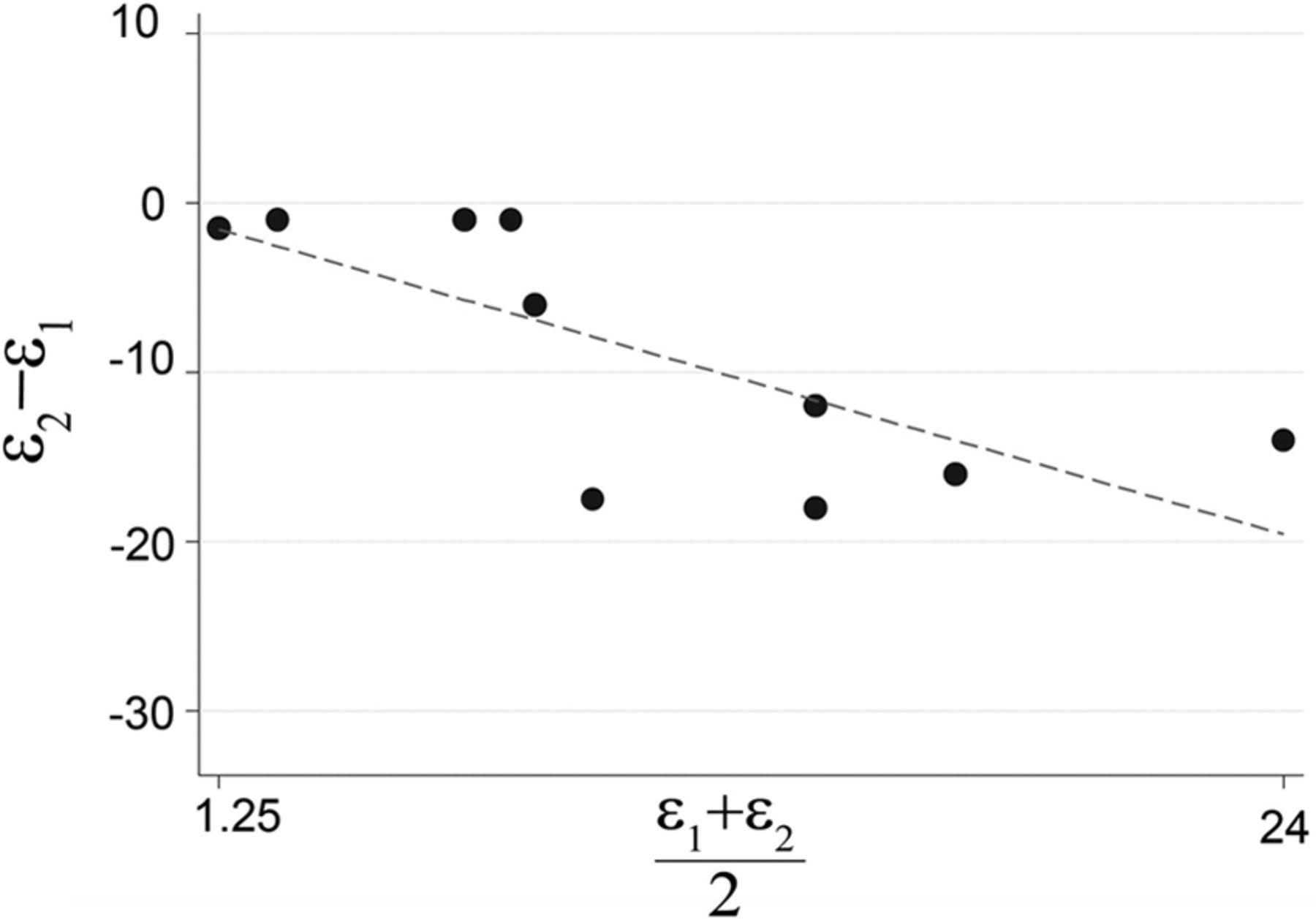
Bland-Altman plots of the WSS on BW for the T0 versus T2 and T0 versus T1 comparison, illustrating significantly higher error for the T2 truncation compared with T1 truncation for all 10 models.
Meaningful Error
To associate the quantitative description with the qualitative observations and define a meaningful error, we compared the contours plots with the error RMS (Equation 4) of the scatterplots representing the magnitudes of T0 versus T1 and T0 versus T2. As an example, Fig 6 shows the results of the WSS on BW for model P1. Here, the contours are visually similar between the T0 and T1 truncations, but slightly different (almost at the border of being different) for the T0 and T2 truncations. In addition, the scatterplot for the aneurysm bleb surface WSS magnitude for the T0 to T1 comparison (Fig 6, lower left) is spread along the 45° diagonal starting from the origin with an error RMS of approximately 17%. The scatterplot for the T0 to T2 comparison for WSS magnitudes on BW (Fig 6, lower right) is more spread out about the diagonal, with an error RMS value of 31%.

WSS magnitude contour plots for the 3 truncations (upper panel) and WSS magnitude scatterplots for the T0 versus T1 comparison and for the T0 versus T2 comparison, respectively (lower panels) for the model P1. The error RMSs defined by Equation 4 corresponding to the 2 scatterplots are 17% and 31%, respectively. The arrows indicate the locations where the area with maximum WSS values diminishes from truncation T0 to truncation T2 and a new area with a local maximum forms in truncation T2.
Another quantitative-qualitative analysis is presented in Fig 7, which shows the contour plots of OSI on BW for model P5 and the scatterplot of OSI values for T0 versus T1 and T0 versus T2 comparisons. In this example, the contours are only borderline slightly different for the T0 to T1 comparison, which is also confirmed quantitatively by the tighter scatterplot of the T0 versus T1 comparison (lower left), with an error RMS of approximately 18%. However, the T2 contour plot is visually different from the T0 contour plot difference, which was more precisely quantified in the scatterplot (lower right), where the points are more widely spread out for higher OSI values with an error RMS value of approximately 54%. The large error RMS could be explained by the location of maximum OSI shifting from the area between the 2 aneurysm blebs in the T0 truncation to an area near the common neck location of the 2 blebs in the T2 truncation (shown with the arrows in Fig 7).

OSI magnitude contour plots on the aneurysm bleb surface for the 3 truncations (upper panels) and OSI magnitude scatterplots on the aneurysm bleb (lower panels). The error RMS defined by Equation 4 corresponding to the 2 scatterplots are 18% and 54%, respectively. The arrow on the T0 contour plot indicates the location of the maximum OSI values, which shifts from the area between the 2 aneurysm blebs in the T0 truncation to an area near the common neck location of the 2 blebs in the T2 truncation.
To find the numeric value of a visually observed meaningful error for all 10 aneurysms, we compared the contour plot results with the error RMS defined in Equation 4, and we found that contour plots with a relative error RMS of <18% could be generally considered qualitatively similar, whereas those with a relative error RMS >32% were associated with qualitatively different contours. Errors between truncations with magnitudes between 18% and 32% were observed to lead to slightly different contours.
Discussion
This is the first study to assess the quantitative differences in the intra-aneurysmal blood flow parameters when truncating the length of the main artery leading to the aneurysm bleb in models of ophthalmic aneurysms and to provide a meaningful error, by associating the quantitative analysis with the qualitative description of hemodynamics results. Usually, visual observations are the standard way to compare the CFD results between models, which can potentially obscure important quantitative differences. To estimate the effect of the arterial length on the flow behavior in the aneurysm bleb, we analyzed the main flow parameters for 10 models, each with 3 truncations: the original maximum length obtained from the patient medical images and 2 user-defined truncations obtained by cutting the ICA artery after each of 2 major turns.
Qualitatively, the visual differences were observed to be small for most of the models when the ICA artery was truncated at the cavernous site (T1 truncations). As such, a simple comparison of the contour plots with our quantitative results showed that the contours could be visually similar for the T0 to T1 comparison, but quantitatively, the average errors could still be relatively large, for example 17% different for WSS in P1 (Fig 6). Because the quantitative differences account for both the location and the magnitude of the hemodynamic parameter investigated, a shifting location of the maximum value on the contour map can be much better assessed with a quantitative description of errors, but it can be sometimes misjudged by visual observation.
When the qualitative differences in the contour plots were compared with the quantitative errors presented in the Table, we observed that errors of less than approximately 18% resulted in visually similar contours for 8 models for the T0 to T1 comparisons. In contrast, for the T0 to T2 comparisons, larger errors were observed for 8 of the 10 models, which resulted in slightly different or different contour plots of the hemodynamic parameters.
In summary, we found that a short arterial truncation, such as T2, at the clinoid segment could generate large quantitative errors and qualitative differences. However, an inlet artery starting at the cavernous segment, as in the T1 truncation, seems to produce qualitatively similar flow behavior, but even for this more modest truncation, the quantitative errors can be too large compared with the flow parameters analyzed for the original model, T0.
Conclusions
When one assesses the accuracy of a computational model for patient-specific aneurysms, quantitative analysis of the hemodynamic parameters must be considered along with visual analysis of the graphic representation of flow quantities. The present study showed that excluding 2 arterial turns from the artery resulted, most of the time, in large quantitative differences of the hemodynamics parameters inside the ophthalmic aneurysm blebs, which could lead to erroneous conclusions if used clinically.
Footnotes
Disclosures: David F. Kallmes—UNRELATED: Board Membership: GE Healthcare, Comments: Cost Effectiveness Board; Consultancy: ev3, Medtronic, Comments: planning and implementation of clinical trials; Grants/Grants Pending: ev3,* Sequent,* Surmodics,* Codman,* MicroVention*; Royalties: University of Virginia Patent Foundation (Spine Fusion). *Money paid to the institution.
REFERENCES
- Received June 30, 2014.
- Accepted after revision September 29, 2014.
- © 2015 by American Journal of Neuroradiology


