
Abstract
BACKGROUND AND PURPOSE: Measurement of the vestibular aqueduct on CT scans of the temporal bone is important for the detection of large vestibular aqueduct syndrome; typically this is done in the axial plane. We sought to determine the usefulness of reformats performed in the 45° oblique plane for evaluating the vestibular aqueduct. In addition, we provide reference measurements for the vestibular aqueduct in the 45° oblique plane.
MATERIALS AD METHODS: We selected 15 subjects referred for reasons other than sensorineural hearing loss, and without radiographic evidence of abnormality of the inner ear. Two neuroradiologists independently evaluated both axial and 45° oblique images for ease in visualizing the vestibular aqueduct. Then, one of the readers (B.O.) performed reference measurements of the diameter at the mouth and midpoint of the aqueduct.
RESULTS: Combining the results of both observers, we judged 82% of vestibular aqueducts as well-defined or easily traced on 45° oblique views, whereas we judged only 55% as well-defined or easily traced on axial views. The difference in the degrees of visualization between the 45° oblique and axial reformats was significant for observer 1 (P =.022) and observer 2 (P =.001). Intraobserver agreement about the visibility of the aqueduct was higher on the 45° oblique than the axial views: (κ = 0.682, SE = 0.171) for 45° oblique reformats; (κ = 0.480, SE = 0.145) for axial reformats. On the 45° oblique reformats, the mean external aperture dimension of the vestibular aqueduct was measured as 0.616 ± 0.133 mm, and the postisthmic segment had a mean width of 0.482 ± 0.099 mm.
CONCLUSIONS: The 45° oblique plane gives a more reliable depiction of the vestibular aqueduct than the axial plane in CT evaluation of the temporal bone. This technique can be useful in cases of borderline enlargement of the vestibular aqueduct.
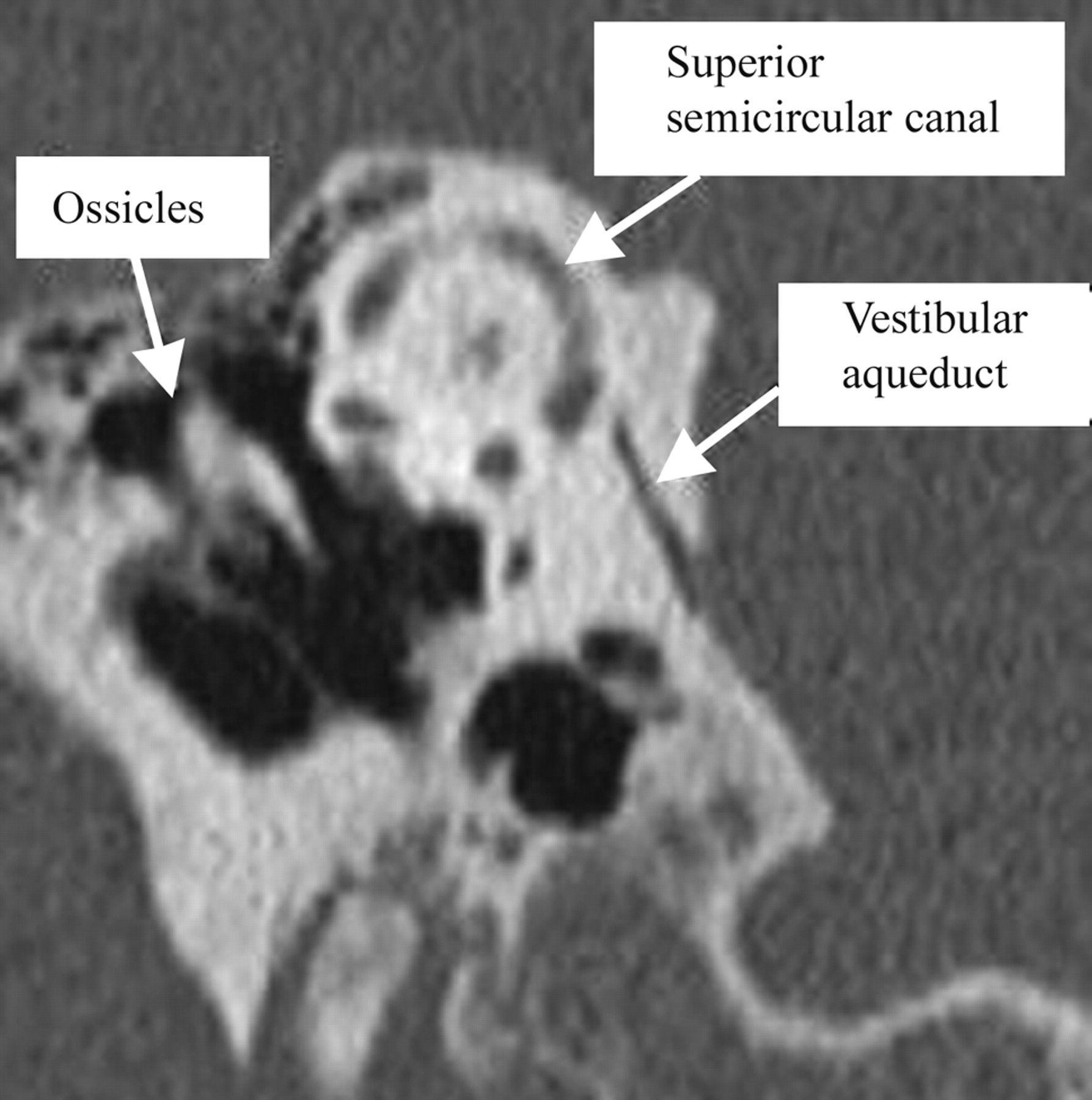
In CT evaluation of children with sensorineural hearing loss, an enlarged vestibular aqueduct is the most commonly detected imaging abnormality.1,2 This diagnosis is made when the diameter of the aqueduct is larger than 1.5 mm at the midpoint of the postisthmic segment.3 Although these measurements are currently taken in the axial plane, previous descriptions and evaluations of the aqueduct with use of pluridirectional tomography (polytomography) were performed in modified lateral and Pöschl projections.3–6 The latter projection, also called the axial projection of the pyramid or the transverse pyramidal plane, was obtained by placing the longitudinal axis of the petrous bone perpendicular to the film and acquiring sections at a right angle to the longitudinal axis of the petrous pyramid.5–7 It was known to demonstrate the entire axis of the aqueduct.6 The Pöschl projection can be replicated in CT imaging of the temporal bone by a sagittal oblique reformat, perpendicular to the axis of the pyramid, or approximately 45° from either the sagittal or coronal planes (Fig 1).8 This reformat is probably most commonly used to depict the entire arc of the superior semicircular canal (SSC) in the evaluation of dehiscence of the SSC.9 However, because this plane is the optimal view for the assessment of the vestibular aqueduct in polytomography, the same principle should apply to the reformats in CT imaging of the temporal bone.5,10 In our study, we evaluated the reliability of the 45° oblique reformats for visualization of the vestibular aqueduct compared with the regular axial reformats and obtained measurements of the normal vestibular aqueduct in the 45° plane.

Reformatted image of a CT of the temporal bone in the 45° oblique plane, demonstrating the position of the vestibular aqueduct.
Patients and Methods
We retrospectively evaluated high-resolution CT studies of the temporal bones performed on 15 patients (30 ears) for reasons other than sensorineural hearing loss. The selected cases demonstrated no radiographic evidence of inner ear abnormality.
CT Scanning
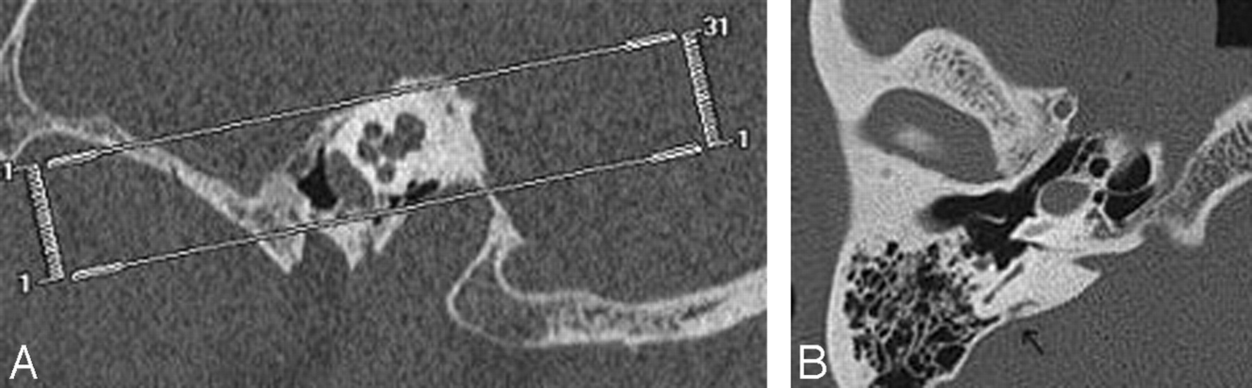
We performed multidetector CT scanning in the axial plane with a 4-channel multidetector CT scanner (SOMATOM Plus 4 Volume Zoom; Siemens, Erlangen, Germany). The images were obtained with 0.5-mm collimation, 0.5-mm thickness, 320 mAs, and 120 kVp. In pediatric patients, we altered the technique to lower the radiation dose by using 120 mAs. We reconstructed the obtained data separately for each temporal bone in the axial plane by using a bone algorithm with 0.5-mm section thickness, 0.5-mm increments, and a FOV of 100, with a matrix size of 512 × 512. At this collimation, we obtained an isotropic voxel, which measures 0.5 mm per side. The axial data were then transferred to a separate workstation for postprocessing, with a commercially available 3D reformatting software (Voxar 3D; Barco, Edinburgh, Scotland). Reformatted images were first made in the axial plane (parallel to the axis of the cochlea on the sagittal view) with a section thickness of 0.8 mm (Fig 2). Then, 45° oblique reformats with 0.8-mm thickness were acquired perpendicular to the petrous pyramid. Because the SSC is located perpendicular to the longitudinal axis of the petrous bone, we determined the 45° oblique plane from an axial scout image to be parallel to the plane of the SSC (Fig 3).11

Planning of the axial reformats based on the sagittal scout image. Axial reformats were obtained parallel to the axis of the cochlea (A). The obtained axial reformat demonstrates the vestibular aqueduct (arrow) (B).

Planning of the 45° oblique reformats based on the axial scout image. The 45° oblique reformats were obtained parallel to the plane of the SSC (A). The obtained reformat demonstrates the vestibular aqueduct (arrow) (B).
Image Evaluation–Grading Conspicuity of the Aqueduct
Two neuroradiologists (B.O., M.E.C.) independently reviewed the 2 sets of reformats (axial and 45° oblique planes) with respect to the visibility of the aqueduct. We used a standardized window/level setting of 4000/800 to display all of the data. We classified the evaluated vestibular aqueducts with a 4-point grading system according to the visibility of the vestibular aqueduct as follows: grade 0, nonvisualized; grade 1, visualized with difficulty/very thin; grade 2, thin but visible; and grade 3, well defined/easily traced (Fig 4).

Grading of the aqueductal visibility. In 1 patient, there is a grade 3 well-visualized aqueduct in both 45° oblique (A) and axial (B) reformats. In another patient, the vestibular aqueduct is judged to be grade 2 (thin but visible) in 45° oblique formats (C), and grade 1 (difficult to see/very thin) on axial reformats (D).
Image Evaluation–Measuring the Postisthmic Aqueduct
We obtained 2 measurements of the aqueduct on each reformat: a measurement at the approximate midpoint and a measurement at the external aperture. We used electronic calipers for all measurements and placed the calipers at the last point which demonstrated bone attenuation by visual inspection of each wall of the aqueduct.
For the measurements at the external aperture, a section which depicted the external aperture in its largest dimension was identified. We then used calipers to draw a line across the aqueduct. Care was taken to make sure the line was as close to the posterior fossa as possible, while still contacting both bony walls (Fig 5).

Measurement of the aqueducts: positioning of the measurement bars at the 2 described levels (midportion of the postisthmic segment and external aperture) in (A) and in axial (B, C) reformats.
The method of obtaining measurement at the midpoint varied between the axial and 45° oblique projections. Valvassori et al.12 measured the vestibular aqueduct at the midpoint of the postisthmic segment, which they defined as “halfway between the external aperture and the common crus.” Further reading of their paper shows that these measurements were performed on tomograms, which had been tailored to demonstrate the common crus and the external aperture in the same plane. It is not always possible to visualize both the external aperture and the common crus simultaneously in the axial plane with thin-section imaging. Therefore, for purposes of this study, we estimated the midpoint by scrolling between the common crus and the external aperture and approximating the midpoint visually (Fig 5).
In the 45° oblique plane, the postisthmic aqueduct can be visualized in 1 section, and we determined the midpoint by visually estimating the halfway point between the external aperture and the common crus (Fig 5).
Results
We evaluated 30 vestibular aqueducts of 15 patients. Of the 15 patients, 8 were male and 7 female, with a mean age of 32.1 ± 24.99 years (range, 3 to 73 years). The patient demographics and indications for which the CT scans were originally obtained are summarized in Table 1.
Patient demographics and indications for temporal bone CT studies
The vestibular aqueducts were visible in all the evaluated temporal bones for both projections. However, the 45° oblique reformats had higher degrees of visualization compared with the axial reformats (Table 2). The difference in the degrees of visualization between the 45° oblique and axial reformats was significant for observer 1 (P = .022) and observer 2 (P = .001) (Wilcoxon test for paired data). On the 45° oblique view, 82% of the 30 evaluated aqueducts were classified as well defined and easily traced (26/30 for observer 1 and 23/30 for observer 2). For the axial plane, the same level of visibility was attained only in 55% of the aqueducts (18/30 for observer 1 and 15/30 for observer 2). The degree of agreement among the 2 observers for evaluating the level of visualization of the aqueducts was judged to be good (κ = 0.682, SE = 0.171) for 45° oblique reformats and moderate (κ = 0.480, SE = 0.145) for axial reformats.
Visibility grade of 30 vestibular aqueducts viewed by 2 readers on 45° oblique and axial reformats
The mean external aperture dimension of the vestibular aqueduct was measured as 0.616 ± 0.133 mm in 45° oblique reformats and 0.742 ± 0.200 mm in axial scans (P = .006, Student t test). In the 45° oblique reformats, the postisthmic segment had a mean width of 0.482 ± 0.099 mm, with a minimum of 0.3 mm and a maximum of 0.73 mm. In the axial plane, the same width had a mean of 0.544 ± 0.119 mm (P = .031, Student t test) (Table 2). The measurements performed from the axial projections were significantly higher than the ones performed from the 45° oblique projections, especially for the measurements at the level of the external aperture but also for the measurements performed from the midportion of the postisthmic segments (P < .006 for the external aperture and P < .03 for the midportion, Student t test) (Table 3). There was a moderate degree of correlation among the midportion measurements performed in the axial and 45° oblique planes (Pearson product moment correlation coefficient, r = 0.525) and among the measurements at the level of the external aperture in both planes (Pearson product moment correlation coefficient, r = 0.527).
Vestibular aqueduct measurements in 45° oblique plane
Comparison of measurements obtained from vestibular aqueducts in axial views (paired Student t test) for both ears
Discussion
The large vestibular aqueduct syndrome was originally discovered during a radiographic study of 3700 patients referred for polytomograms performed by Valvassori and Clemis.3 These authors described 50 patients who had a vestibular aqueduct greater than 1.5 mm in diameter. Of these 50 patients, 29 demonstrated other temporal bony anomalies; 21 demonstrated a large vestibular aqueduct as an isolated finding. Subsequently, the clinical entity associated with isolated enlargement of the vestibular aqueduct was described.13–15 Patients demonstrated progressive hearing loss in childhood and were at risk of sudden hearing loss with mild trauma. The identification of a distinct clinical syndrome associated with the anatomic finding of an enlarged vestibular aqueduct elevated the importance of detecting this abnormality on imaging.
The anatomy of the vestibular aqueduct is well described in the literature.3–5,10,11,16–18 In an adult, the vestibular aqueduct has an inverted J appearance with a short ascending proximal segment and a longer distal descending segment. The proximal segment arises from the medial wall of the vestibule and curves superiorly and medially up to a bend. As it runs parallel to the common crus formed by the superior and posterior semicircular canals, its length and shape are fairly constant.17 This segment includes the narrowest portion of the aqueduct, called the isthmus, corresponding to the bend. The distal straight segment enlarges along its inferior and posterior course and ends as the external aperture on the posterior surface of the petrous pyramid. The postisthmic segment of the vestibular aqueduct is shaped like a compressed cone with a flattened oval cross section.3 The long diameter of the oval runs anteromedial to posterolateral. The short axis runs anterolateral to posteromedial. The vestibular aqueduct is considered enlarged when the shorter, anterolateral-to-posteromedial diameter measures greater than 1.5 mm.3
In their study, Valvassori and Clemis3 measured the vestibular aqueduct on modified lateral tomograms. Since that time, CT has replaced pluridirectional tomography and became the primary method for the evaluation of the temporal bone.19 Before the advent of multidetector CT, projections such as the 45° oblique plane would have required very difficult head positioning on the CT scanner. It is not surprising that most of the reported data on the CT imaging of the vestibular aqueduct were based on measurements obtained on the routine axial sections.2,19,20
However, the postisthmic segment of the aqueduct has an approximately 70° angulation from the routine axial plane (Fig 6). Two problems arise as a result of this angulation. First, the vestibular aqueduct cannot be seen in its entire length on a single axial section. This shortcoming may interfere with visualization of the aqueduct and cause diagnostic challenges.21

Diagram demonstrating the plane of the axial image across the vestibular aqueduct on the 45° oblique reformat. A line is drawn connecting 2 points of the lateral semicircular canal. This line demonstrates the obliquity of the axial reformat to the axis of the vestibular aqueduct.
The second problem that arises because of the 70° angulation of the aqueduct from the axial imaging plane is a potentially artifactually enlarged measurement of the diameter of the aqueduct. In any cylindrical or conical structure, the shortest diameter at any level will be obtained by taking a measurement perpendicular to the central axis of the structure. This is only possible if the plane of the image is parallel or perpendicular to this central axis. Measurements of the aqueduct on the axial images will usually be oblique with respect to the long axis, rather than perpendicular, and therefore the cross section will be artifactually enlarged. Our data support this finding: the diameter measurements in the axial plane are significantly larger. Because an enlarged vestibular aqueduct is often the only anomaly identified in a patient with sensorineural hearing loss, precise measurement is required. Of course, in many patients the aqueduct is grossly enlarged and easily identified as such, regardless of the projection. Increased precision of measurement is most valuable in borderline cases.
Currently, with the widespread use of multidetector spiral CT scanners, the acquired images can be reformatted in any desired plane with identical spatial resolution.22 On the basis of previous tomographic experience, some authors suggested the use of direct or reformatted sagittal CT images2,12,20 for evaluation of the vestibular aqueduct. However, tomographic studies have reported that the 45° oblique projection gives a better visualization of the vestibular aqueduct compared with the lateral (sagittal) projection.10 Most of the earlier articles published in the tomographic literature recommend true lateral or off-lateral projections for the evaluation of the vestibular aqueduct.11,23 Valvassori3,6 suggested the use of axial projection of the pyramid (45° oblique projection), in addition to the sagittal projection because this projection exposes the long axis of the aqueduct in its full extent. Korach5 also emphasized the importance of the 45° oblique projection in the demonstration of the aqueduct. In a similar fashion, Becker et al4 have found that the axial projection of the pyramid is of great value in the evaluation of the vestibular aqueduct in congenital deafness.
In the CT literature, coronal images have also been suggested for evaluation of the vestibular aqueduct. However, coronal images also are significantly angulated from the axis of the aqueduct and, not surprisingly, coronal measurements of the aqueduct are slightly larger than the previously reported anatomic measurements.21 Murray et al21 have reported 100% identification and measurability of the vestibular aqueduct in the coronal plane. In our study, although the vestibular aqueducts of all patients could be identified in both planes, the aqueducts imaged in the 45° oblique plane had a higher grade of visibility (and easier identification) than the ones imaged on the axial scans. Furthermore, the impressions of both observers were such that even in cases in which the aqueducts were more difficult to identify, they could be traced more easily on the 45° oblique plane.
The appearance of the aqueducts in the 45° oblique reformats was in agreement with the previously described course of the aqueduct. The progressive minimal widening of the post- isthmic segment and the triangular opening at the external aperture were well depicted. The mean of the measurements performed from the postisthmic segment at its midpoint was 0.482 mm (±2 SD) in 45° oblique reformats with a minimum width of 0.3 mm and a maximum of 0.73 mm. The mean width of the external aperture was 0.616 mm (range, 0.4–0.85 mm). These measurements correlate well with previously reported aqueduct dimensions obtained from anatomic specimens.11,17 As discussed, the measurements performed from the axial planes were significantly higher than the ones performed from the 45° oblique planes.
Conclusion
Because of its oblique orientation, the aqueduct has always been challenging for radiographic demonstration. In the past, the 45° oblique projection, taken perpendicular to the petrous apex, had provided the best view of the aqueduct on tomograms of the temporal bone. With application of the same principle to modern CT imaging of the temporal bone, 45° oblique reformats can easily be obtained without any loss of resolution. This reformat provides a better visualization compared with routine images in the axial plane and also allows more accurate measurement of the aqueduct in a fashion that mimics the method in which the measurements were originally made on polytomograms.
It should be stated that very enlarged aqueducts can be easily seen on axial views, and we do not obtain 45° oblique reformats in cases of grossly enlarged vestibular aqueducts. The value of this technique lies in the analysis of borderline cases. Our data suggest that measurements made in the 45° oblique plane would allow some equivocally enlarged aqueducts to be more definitively classified as normal.
References
- Received December 14, 2006.
- Accepted after revision May 24, 2007.
- Copyright © American Society of Neuroradiology


