
From its very beginning, MR as an imaging method suffered from inherently low signal intensity. A typical way to compensate for low signal intensity is the repetition of measurements, which causes long imaging times. Besides that, a variety of different approaches are used to increase signal intensity. Gradient systems have been substantially improved for new sequences with higher intrinsic signal intensity, for example in steady-state sequences like trueFISP (1). Radio-frequency (RF) coil design has advanced to arrays of smaller coils (2), which also improve the signal intensity. Contrast media for special applications have also been developed (3–5) to increase MR signal intensity. Although these developments are independent of field strength, the advance of a new generation of MR scanners with higher B0 fields opens another approach to substantially increase signal intensity (6, 7). These scanners have recently become more widely available in clinical routine diagnostics (6). Increased signal intensity, however, is not the only effect of higher field strength (7–11), and associated effects necessitating changes in acquisition strategies have lead to a debate about the usefulness of higher field strength in clinical settings (12–14). The focus of this review is to illustrate some of the effects and limitations of higher B0 imaging providing imaging examples from neuroradiologic applications and practical considerations on how to overcome some of these limitations.
Theoretical Advantages and Disadvantages of MR Imaging at 3T
Signal Intensity-to-Noise Ratio
In theory, the intensity of MR signal is linearly correlated with the strength of the static magnetic field B0 (7). When compared with common methods of signal intensity enhancement (eg, increasing the number of excitations [NEX]), higher B0 strength appears to be of clear advantage. Although relative signal intensity increase is linearly correlated with B0, it follows the square root of NEX only—ie, to achieve doubling in signal intensity at constant B0 necessitates a 4-fold increase in acquisition time (Fig 1).

Comparison of the theoretical signal intensity increase when increasing NEX (gray line) or field strength (B0, black line). To reach the same signal intensity one can get from the doubling field strength, the acquisition time is 4 times longer (circles). Numbers along the x axis refer to levels of NEX and B0, respectively.
Larmor Frequency, Wavelength, and Specific Absorption Ratio
There are some effects associated when moving to higher field strength that, at first glance, appear to be counterproductive. The main problem is the increase in excitation frequency ω according to the Larmor equation: 
Where γ denotes the gyromagnetic ratio (42.58 MHz/T) and B the magnetic field strength. Therefore, the resonance frequency increases from approximately 63.9 MHz at 1.5T to 127.8 MHz at 3T. For calculating the wavelength λ in water (speed of light λ0 = 300.000.000 m/s divided by resonance frequency), one has to take the dielectric constant of water (ε = 81) into account: 
It follows that wavelength λ in water is reduced from 52 cm at 1.5T to 26 cm at 3T (7). The shorter wavelengths are substantially closer to natural body diameters, which results in an increase of shielding effects and interferences (15) from superimposed RF waves with complex effects on RF homogeneity (16). The associated problems are most obvious in abdominal and pelvic imaging. Possible solutions like RF shimming and improved coil design (17) are being evaluated (18).
Energy deposition in terms of specific absorption ratio (SAR) relates to the square of excitation frequency, which means that problems with SAR limitations scale with the square of B0 field strength (Fig. 2).

Theoretic increase in relative signal intensity for NEX and field strengths B0 (gray lines) as in Fig 1. Note the relative increase in SAR related to field strength (black line). Although signal intensity linearly increases with field strengths, SAR increases with the square of field strengths. Values on the y axis are arbitrary units solely to demonstrate the relationship between the increases of different parameters in one graph.
Relationship between Chemical Shift, Bandwidth, Signal Intensity, and SAR
Effects of chemical shift scale linearly with B0. Therefore, fat and water resonance frequencies differ by 220 Hz at 1.5T and 440 Hz at 3T (19). Moreover, chemical shift (CS) is inversely related to the receiver bandwidth (BW, in Hz/pixel): 
From the relation above, it follows that compensation for chemical shift effects at 3T is possible by measuring with doubled bandwidth at 3T relative to 1.5T (Fig 3). Signal intensity, however, is inversely related to the square root of bandwidth (19): 
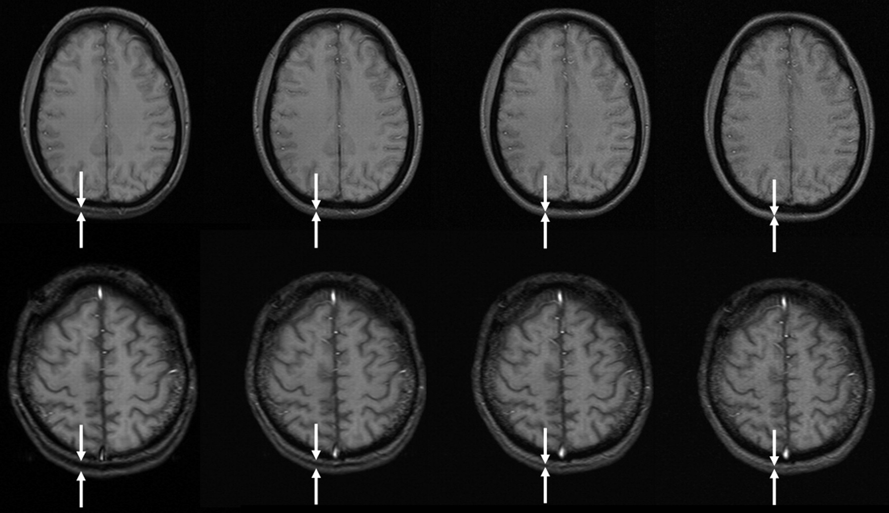
Chemical shift artifacts at different bandwidths at 1.5 (upper row: TR, 172 ms; TE, 9 ms; field of view [FOV], 220 × 220 mm2; matrix, 256 × 192) and 3T (lower row: TR, 206 ms; TE, 10 ms; section thickness, 5 mm; FOV, 220 × 220 mm2; matrix, 256 × 192). Bandwidth increases from left to right (60, 120, 240, 480 Hz/pixel), resulting in chemical shift of 7.4, 3.7, 1.9, and 0.9 pixels, respectively, at 3T, and half of these values at 1.5T. Note the double line of the occipital subcutaneous tissue at lower bandwidths (between white arrows). Of note also is the increasing noise at higher bandwidths.
Consequently, increasing bandwidth reduces part of the extra signal intensity provided from imaging at 3T. In other words, doubling bandwidth to keep chemical shift effects constant between 1.5T and 3T reduces the original signal intensity gain obtained from 3T when compared with 1.5T from 200% to 141%.
Unfortunately, a higher bandwidth aggravates the problem of SAR exposure, but, because numerous other factors—including type and number of RF pulses, flip angle, number of sections, echo train length, sequence design, coil design, patient positioning, number of sections, and additional pulses for fat saturation—affect SAR as well, a general prediction is not adequate.
Altogether, compensating increased chemical shift at 3T by means of increasing bandwidth appears to be an unsatisfactory solution. Because chemical shift is not a severe problem in brain imaging, larger shifts between water and fat can probably be tolerated. For other body regions, however, compensating mechanisms such as fat suppression are more often necessary.
Practical Considerations Combined with Imaging at 3T
Solutions for SAR Problems at Higher Field Strengths
An effective approach to reduce SAR problems at higher fields is related to changes of the excitation or refocusing flip angle. Because energy deposition is proportional to the square of flip angle (20), even small reductions of the flip angle lead to significant SAR decreases. Most technicians and radiologists, however, are unsure about how flip angle variations may affect image contrast and therefore refrain from changing this parameter. Moreover flip-angle reductions (21) may involve a reduction in signal intensity, limiting the gain from higher field.
New sequences using hyperechoes (22) make use of the effect that only the central k space is relevant for image contrast (23). Consequently, these sequences automatically narrow the excitation flip angles only for the outer k-space lines while exciting the central k space with higher flip angles to achieve contrast (Fig 4).

T2 turbo spin-echo (left) and hyperecho (right) of the same section position and with all other parameters kept equal (TR, 3810 ms; TE, 78 ms; matrix, 832 × 416; FOV, 220 × 220 mm2; echo train length [ETL] 9; section thickness, 5 mm; bandwidth, 145 Hz/pixel; flip angle, 120°), demonstrating that there is no difference in image contrast while SAR was significantly reduced.
The use of gradient echo sequences is a valuable alternative (Fig 5) to the approach discussed above to significantly reduce SAR. These sequences, however, are prone to susceptibility artifacts especially at higher B0 and longer TE, limiting their use at 3T.

Gradient echo T1 (left: TR, 311 ms; TE, 2.5 ms; section thickness, 5 mm; matrix, 512 × 256; FOV, 220 × 220 mm2; bandwidth, 465 Hz/pixel; flip angle, 90°) compared with T1 spin-echo (right: TR, 700 ms; TE, 10 ms; section thickness, 5 mm; matrix, 256 × 192; FOV, 220 × 220 mm2; bandwidth, 200 Hz/pixel; flip angle, 90°) in the same subject at 3T, which indicates higher contrast in gradient echo than spin-echo sequences at 3T.
Very promising approaches are parallel imaging techniques (24–29) that permit the carry over of signal intensity to speed. The underlying concept is the reduction of phase encoding steps necessary for image acquisition. By this, the number of excitation pulses is reduced, thereby decreasing SAR. SNR, however, also decreases by the very same mechanism. So, for example, to achieve the same SAR level at 3T one yields at 1.5T, a speed-up factor of 4 is needed. This speed-up factor reduces SNR by 50%. Consequently, for this example, one ends up with the same SAR, the same resolution and the same SNR one can get from 1.5T, but acquisition is 4 times faster. Unfortunately, parallel imaging does not yet primarily turn signal intensity increase into higher spatial resolution.
T1 Spin-Echo Contrast
Apparently, gray-to-white matter contrast is reduced in spin-echo T1 imaging at 3T (30) when compared with 1.5T (Fig 6). There are several factors contributing to this observation. T1 times of gray and white matter lengthen and converge at higher fields (31–33). Moreover, shielding effects induced by eddy currents prevent central parts of the image from being properly excited (16), which results in reduced signal intensity of the basal ganglia region. In addition, magnetization transfer effects are enhanced at higher B0, thus reducing signal intensity and contrast. There are several ways to compensate for these effects. For example, inversion recovery sequences appear very well suited if one is only interested in increasing gray to white matter contrast (Fig 7). The inversion pulse, however, interferes with visualization of contrast enhancement following gadolinium administration. Enhancing lesions may not be visible (Fig 8), because in inversion recovery sequences, unlike conventional T1 spin-echo sequences, the tissue with the shortest T1 does not necessarily exhibit the brightest signal intensity, depending on T1. Therefore, inversion recovery sequences are not quite useful for comparative pre- and postcontrast T1 spin-echo imaging, regardless of B0. A different approach to increase gray-to-white matter contrast during T1-weighted spin-echo imaging at both field strengths is to reduce the excitation flip angle (34). Although this reduces SNR slightly, the gain in gray-to-white matter contrast is obvious and more pronounced at 3T (Fig 9). The effect can be predicted from theoretical calculations (35) by using known T1 and T2 relaxation times of gray and white matter (33) but is empirically larger than the theoretical predictions at 3T, probably because of shielding and magnetization transfer effects (34).

Left, T1 spin-echo image at 1.5T (TR, 600 ms; TE, 14 ms; bandwidth, 90 Hz/pixel; section thickness, 5 mm; matrix, 256 × 192; FOV, 220 × 220 mm2; flip angle, 90°). Right, T1 spin-echo at 3T (TR, 700 ms; TE, 10 ms; section thickness, 5 mm; 19 sections; bandwidth, 200 Hz/pixel; matrix, 256 × 192; FOV, 220 × 220 mm2; flip angle, 90°), which is indicative of the reduced gray-to-white matter contrast at higher fields.

Turbo inversion recovery (TIR) sequence at 1.5T (left: TR, 8770 ms; TE, 92 ms; TI, 300; matrix, 512 × 256; section thickness, 3 mm; FOV, 220 × 220 mm2; bandwidth, 130 Hz/pixel) and 3T (right: TR, 8890 ms; TE, 95 ms; TI, 300; all other parameters equal), which demonstrates clear depiction of gray and white matter at both field strengths.

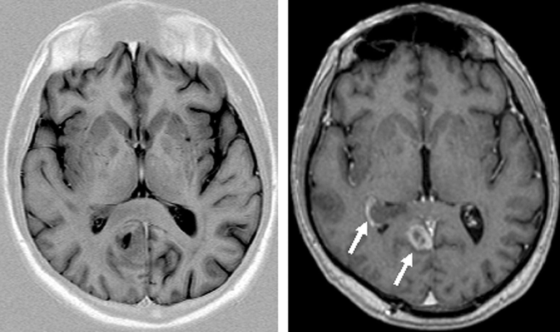
Same axial section position of a TIR (TR, 7670 ms; TE, 68 ms; TI, 300; ETL, 15; matrix, 448 × 224; section thickness, 4.5 mm; bandwidth, 130 Hz/pixel; flip angle, 150°) and T1 sequence (magnetization-preparation rapid gradient echo TR, 1880 ms; TE, 3.7 ms; matrix, 256 × 230; FOV, 256 × 256 mm2; section thickness, 5 mm, reconstructed from 1.0 mm primarily; bandwidth, 160 Hz/pixel; flip angle, 8°) after contrast agent in a patient with a contrast-enhancing lesion. Note the absent contrast enhancement in the TIR image (white arrows in the T1 image).
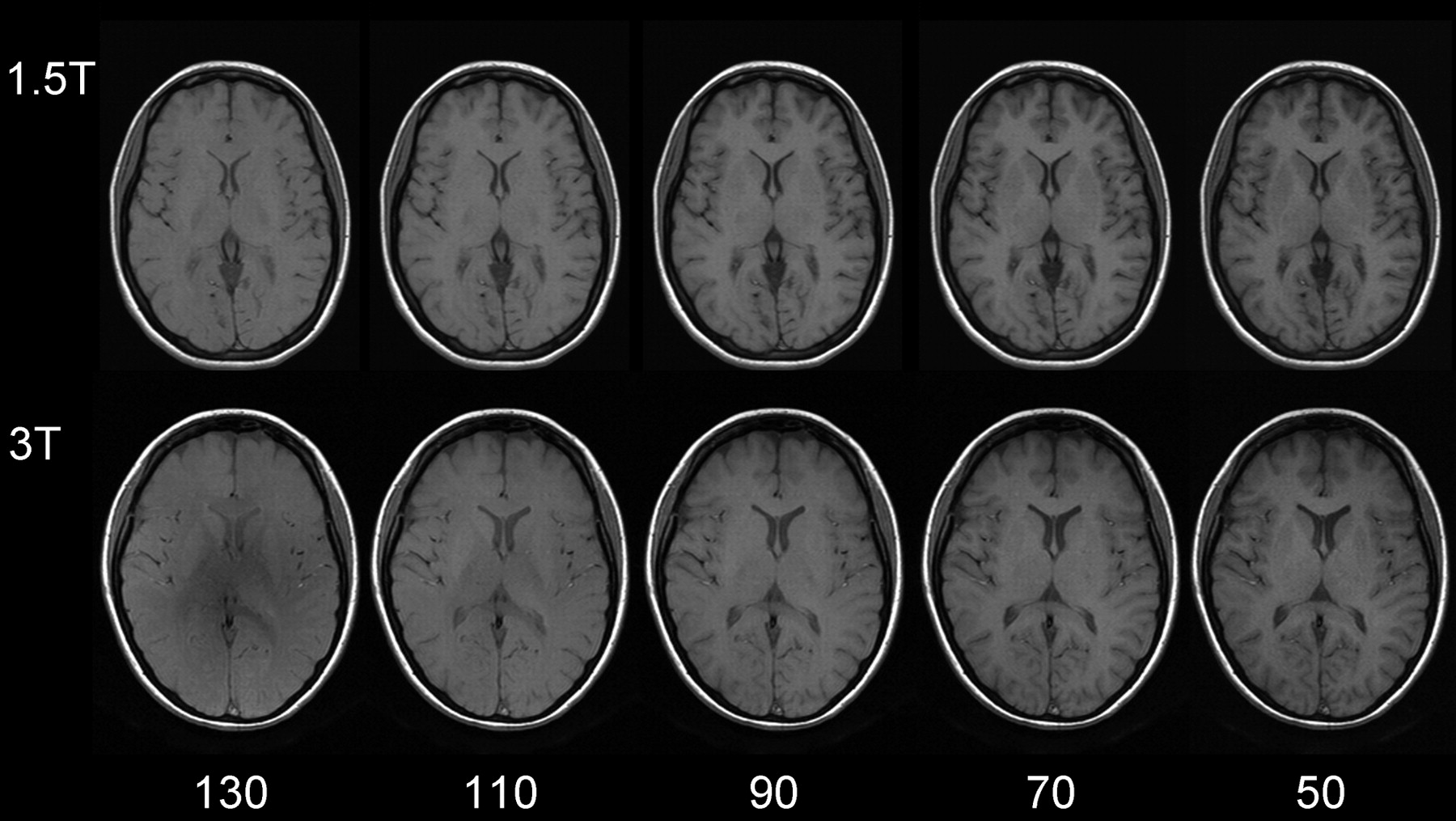
Same section position with spin-echo T1-weighted sequences at 1.5T (upper row: TR, 700 ms; TE, 10 ms; section thickness, 5 mm; matrix, 256 × 192; FOV, 220 × 220 mm2; bandwidth, 200 Hz/pixel) and 3T (lower row: same imaging parameters). Flip angles decreasing from left to right 130°, 110°, 90°, 70°, 50°. The lowest flip angle shows the best gray-to-white matter contrast. The effect is stronger at higher field.
Susceptibility Effects at Higher Field Strength
Susceptibility effects increase with higher B0. Although this can cause artifacts, it is also of clear advantage for susceptibility-related imaging such as T2* sequences for detection of hemosiderin (Fig 10) relevant for detection of microbleeding in vascular encephalopathy (36). Cerebral hemorrhage is reliably detected at 3T (37).

Patient with multiple cavernomas inducing large susceptibility artifacts in T2* imaging at 3T, which is indicative of the high sensitivity for susceptibility effects at 3T (TR, 800 ms; TE, 26 ms; flip angle, 20°; bandwidth, 80 Hz/pixel; section thickness, 5 mm; matrix, 320 × 320; FOV, 220 × 220 mm2).
Functional MR Imaging at Higher Field Strength
Functional MR imaging (fMRI) clearly benefits from higher field strengths (38–41). Because of increased susceptibility effects at 3T BOLD (blood oxygen level–dependent) signals increase with higher B0 (Fig 11). Artifacts at air-bone interfaces can, however, be substantially aggravated at higher field strength, and their dependence from echo times (TE) at 3T is more apparent than at lower magnetic field strengths.

Empirical data from a blocked finger tapping fMRI study at 1.5T and 3T comparing BOLD signal intensity strength in terms of statistical effect sizes (beta values from a linear regression equation; units are arbitrary) at different TEs (54 volumes scanned, a stimulus onset asynchrony of 16 volumes, and an epoch length of 8 volumes. Beta values were computed from scaled episeries within the general linear model by using SPM 99). There is a more than linear increase in BOLD signal intensity with higher field strength.
To achieve the same BOLD signal intensity at 1.5T and 3T, one can use a markedly shorter TE at 3T. In turn, shorter TE permits shorter acquisition times and gives the possibility to increase the number of repetitions. Consequently, it is possible to increase the temporal resolution for fMRI (higher sampling rate of the hemodynamic response function) or increase the statistical power for signal intensity analyses. It is important to bear in mind that shorter TE are very useful in solving the problem of distortions at the skull base, which increase with increasing B0 because of an increase of susceptibility effects in T2*-weighted imaging (Fig 12).

Comparison of susceptibility artifacts at the skull base for 1.5T and 3T at different TEs, keeping all other parameters equal (TR, 4500 ms; isotropic voxel size, 3.3 mm; 48 sections; bandwidth, 2170 Hz/pixel). Artifacts are larger at any TE for 3T and increase with rising TE for both field strengths. At low TE, however, skull base artifacts are tolerable at 3T.
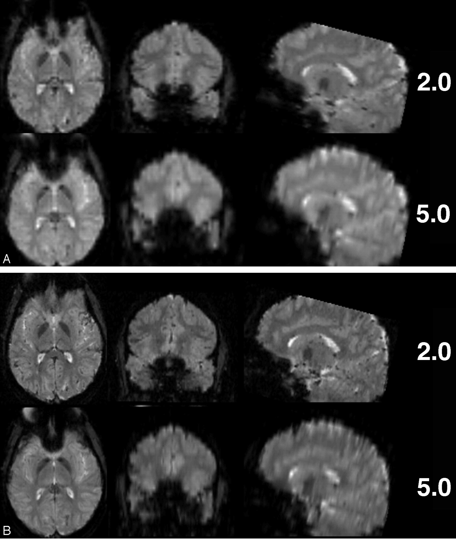
Further handles for optimizing echoplanar sequences to control for distortion effects at 3T are bandwidth and echo spacing (Fig 13). Reducing section thickness or increasing in-plane resolution (eg, 128 × 128 matrices) are additional options of note (Fig. 14A, -B).

Same section position in axial EPI images of the same subject (TR, 4090 ms; TE, 54 ms; isotropic voxel size, 3.3 mm; 36 sections at 3.0T). Decrease of susceptibility effects with increasing bandwidth (in Hz/pixel) due to shorter echo spacing and duration of EPI readout. At low bandwidths (752 Hz/pixel, in this example), distortion effects from the frontal sinus are clearly obvious; however, very high bandwidths (4882 Hz/pixel) do not yield a significant further reduction of distortions that are already achieved with bandwidths at 2520 Hz/pixel.

Comparison of EPI with different voxel size regarding susceptibility artifacts at 3T. (A) Thinner sections (matrix, 64 × 64; TR 4500 ms; TE, 38 ms; bandwidth, 2170 Hz/pixel; FOV, 190 × 190 mm2; 53 sections; section thickness, 2 and 5 mm) and (B) smaller in-plane voxel sizes (matrix, 128 × 128; all other parameters same as in A) result in fewer susceptibility artifacts, especially in frontobasal regions.
MR Angiography at Higher Field Strength
MR angiography (MRA) is one of the most significantly improved MR techniques at higher field strength (42–46). Regarding time of flight (TOF) imaging (Fig 15), longer T1 times at 3T have the effect that the signal intensity inside the vessels is preserved even with thicker sections and in smaller vessels. Moreover, SNR is significantly increased, making higher resolutions possible within reasonable acquisition times (47). This results in better diagnostic quality—for example, with respect to intracranial aneurysms (48, 49).
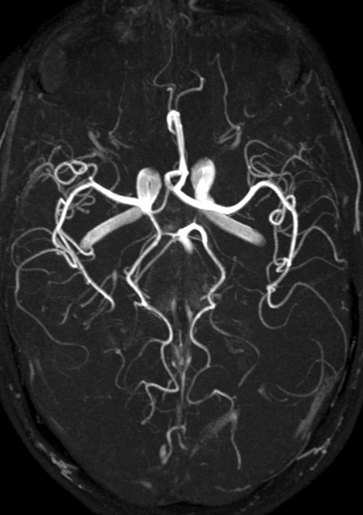
Maximum intensity projection of a time-of-flight angiography (TR, 28 ms; TE, 4.92 ms; matrix, 704 × 576; FOV, 163 × 200 mm2; 92 sections; section thickness, 0.75 mm; bandwidth, 105 Hz/pixel; flip angle, 25°) at 3T showing the clear depiction of even very small vessels.
Conclusion
MR imaging at 3T offers new potential because of a substantial increase in signal intensity provided by the higher magnetic field; however, associated changes—including increased SAR exposure, changed T1 and T2 relaxation times, decreased T1 tissue contrast, and increased susceptibility effects—render high-field MR imaging more compelling. Routine neuroradiologic imaging is feasible and may benefit from higher magnetic field strength, but appears to be more complicated than at lower field strength, and requires extended knowledge of the physical and technical requirements of MR imaging.
Footnotes
This work was presented in abstract form at the 90th scientific assembly and annual meeting of the Radiological Society of North America, November 28–December 3, 2004, Chicago, IL.
References
- Received February 19, 2005.
- Accepted after revision April 18, 2005.
- Copyright © American Society of Neuroradiology
In this issue


Jump to section
Related Articles
Cited By...
- Diagnostic Performance of TOF, 4D MRA, Arterial Spin-Labeling, and Susceptibility-Weighted Angiography Sequences in the Post-Radiosurgery Monitoring of Brain AVMs
- Clinical and Pathophysiologic Correlates of Basilar Artery Measurements in Fabry Disease
- High-Resolution MRA Cerebrovascular Findings in a Tri-Ethnic Population
- Assessment of Heating on Titanium Alloy Cerebral Aneurysm Clips during 7T MRI
- Comparison of structural MRI brain measures between 1.5T and 3T: data from the Lothian Birth Cohort 1936
- Brain Tumor-Enhancement Visualization and Morphometric Assessment: A Comparison of MPRAGE, SPACE, and VIBE MRI Techniques
- Susceptibility-Weighted Angiography for the Follow-Up of Brain Arteriovenous Malformations Treated with Stereotactic Radiosurgery
- Comparison of Dynamic Contrast-Enhanced 3T MR and 64-Row Multidetector CT Angiography for the Localization of Spinal Dural Arteriovenous Fistulas
- Blood Flow of Ophthalmic Artery in Healthy Individuals Determined by Phase-Contrast Magnetic Resonance Imaging
- Can 3T MR Angiography Replace DSA for the Identification of Arteries Feeding Intracranial Meningiomas?
- High-Resolution 3D-Constructive Interference in Steady-State MR Imaging and 3D Time-of-Flight MR Angiography in Neurovascular Compression: A Comparison between 3T and 1.5T
- Normal Pituitary Stalk: High-Resolution MR Imaging at 3T
- 3T MR Imaging of Postoperative Recurrent Middle Ear Cholesteatomas: Value of Periodically Rotated Overlapping Parallel Lines with Enhanced Reconstruction Diffusion-Weighted MR Imaging