
Abstract
BACKGROUND AND PURPOSE: Accurate determination of glioma grade leads to improved treatment planning. The criterion standard for glioma grading is invasive tissue sampling. Recently, radiomic features have shown excellent potential in glioma-grade prediction. These features may not fully exploit the underlying information in MR images. The objective of this study was to investigate the performance of features learned by a convolutional neural network compared with standard radiomic features for grade prediction.
MATERIALS AND METHODS: A total of 237 patients with gliomas were included in this study. All images were resampled, registered, skull-stripped, and segmented to extract the tumors. The learned features from the trained convolutional neural network were used for grade prediction. The performance of the proposed method was compared with standard machine learning approaches, support vector machine, random forests, and gradient boosting trained with radiomic features.
RESULTS: The experimental results demonstrate that using learned features extracted from the convolutional neural network achieves an average accuracy of 87%, outperforming the methods considering radiomic features alone. The top-performing machine learning model is gradient boosting with an average accuracy of 64%. Thus, there is a 23% improvement in accuracy, and it is an efficient technique for grade prediction.
CONCLUSIONS: Convolutional neural networks are able to learn discriminating features automatically, and these features provide added value for grading gliomas. The proposed framework may provide substantial improvement in glioma-grade prediction; however, further validation is needed.
ABBREVIATIONS:
- CNN
- convolutional neural network
- GB
- gradient boosting
- ML
- machine learning
- SVM
- support vector machine
- RF
- random forest
- T1CE
- T1 contrast-enhanced
Primary CNS tumors originate from cells within the CNS and can be benign or malignant.1 Malignant brain tumors require aggressive therapies and are the most challenging to treat. Gliomas are the most frequent malignant primary brain tumors in adults, with an incidence of approximately 5–10 per 100,000 in the population every year.2 Gliomas are divided into low-grade and high-grade gliomas. The prognosis for high-grade glioma is poor, despite treatment options including chemotherapy, radiation therapy, and surgery.3 The 5-year relative survival rate after diagnosis of a brain tumor is 35.8%, with the most aggressive grade IV glioblastoma multiforme having the lowest survival rate of 6.8%.4 In addition, treatment strategy depends on the glioma grade.5,6 While clinical glioma grading is still based on histopathologic methods from tissue sampling, an accurate and reliable noninvasive imaging-based determination of glioma grade is desirable.
Gliomas are classified as grades I–IV, according to the World Health Organization Classification of CNS tumors.7 Glioma grades were restructured in the 2016 version of the World Health Organization Classification, considering molecular information along with the histology.8
Recently, there have been several studies showing the potential for a noninvasive method of glioma grading using radiomic features extracted from MR images. A histogram-based texture analysis was performed by Skögen et al9 on 95 patients to differentiate low-grade from high-grade gliomas. This study reported a receiver operating characteristic area under the curve of 0.910. In another study to classify grades II–IV, Tian et al10 performed texture analysis in 153 patients using a support vector machine (SVM) model reporting an accuracy of 98%. This study also showed that the contrast-enhanced T1-weighted (TICE) method yields the best sequence for grade prediction. Xie et al11 were able to differentiate grade III and IV and grade II and III gliomas using entropy and inverse difference moment of model-free and dynamic contrast-enhanced MR imaging.
These prior MR imaging–based glioma grading studies used hard-coded features that are straightforward to extract. We hypothesized that such an approach limits the use of rich information embedded in the multicontrast MR images. The premise of this work is that rich imaging information beyond simple changes in image contrast/intensity is the following; 1) deeply embedded in pre- and postcontrast enhanced MR imaging, 2) potentially valuable in glioma grading, and 3) learned from labeled training data using deep learning techniques.
In recent years, convolutional neural networks (CNNs) have shown superior performance in numerous visual object-recognition and image-classification studies.12 They also accelerated the development of medical image analysis,13 including applications for tumor diagnosis.14 With a CNN, a hierarchy of features can be learned from a low to high level in a layer-by-layer manner.15 Recently, CNNs15 have also been used for glioma classification. Ertosun and Rubin16 proposed a CNN to classify glioma grades (II, III, and IV) and low-grade-versus-high-grade gliomas, obtaining accuracies of 71% and 96%, respectively. Anaraki et al17 proposed a CNN and genetic algorithm to classify glioma grades (II, III, and IV), obtaining an accuracy of 90.9%. Yang et al18 explored a transfer-learning approach for glioma grading, obtaining 90% test accuracy. However, all of these studies lacked a sufficiently large dataset from which features could be learned.
In this study, we propose a CNN to predict glioma grade from pre- and post-contrast-enhanced MR images. We automatically learn features by training a supervised deep network. The learned features are used for classification and are compared using machine learning (ML) approaches that are trained using radiomic features alone.
MATERIALS AND METHODS
Imaging Dataset
Clinical data were obtained from patients with a diagnosis of glioma who received standard of care brain MR imaging with and without a gadolinium-based contrast agent at the Keck Medical Center of the University of the Southern California from May 2007 to January 2019. Retrospective data were obtained under a protocol approved by the University of Southern California institutional review board (protocol HS-19–00019). The patients were imaged by using a 3T MR imaging scanner (GE Healthcare). The imaging acquisition protocol was the same for all patients and included the following sequences: T1-weighted (TR = 700 ms; TE = 10 ms; flip angle = 90°; section thickness = 5 mm; spacing between slices = 7 mm), T1CE (TR = 500 ms; TE = 19 ms; flip angle = 90; section thickness = 5 mm; spacing between slices = 7 mm), T2-weighted (TR = 5000 ms; TE = 100 ms; flip angle = 90°; section thickness = 5 mm; spacing between slices = 7 mm), and T2-weighted/FLAIR (TR = 8802 ms; TE = 158 ms; flip angle = 90°; section thickness = 5 mm; spacing between slices = 7 mm).
Preprocessing
The dataset contained 366 adult patients with a total of 1154 scans. Because of poor image quality or unknown pathology, 65 patients were excluded from the study. The remaining 301 patients with 887 scans qualified for the study. First, all images were resampled to 1-mm3 isotropic resolution using BrainSuite software (http://brainsuite.org/).19 Second, the 4 volumes were coregistered using the FSL (http://www.fmrib.ox.ac.uk/fsl) toolbox.20 Third, images were skull-stripped using BrainSuite software.19 Forty-two patients were excluded due to skull-stripping failure, leaving 259 patients’ scans to undergo further segmentation.
A fully-automated brain tumor segmentation tool was used to identify lesion regions (enhancing tissue, nonenhancing tissue, and edema) from the skull-stripped multimodal images. This algorithm was one of the top-performing tools as evaluated in the international 2017 Multimodal Brain Tumor Segmentation challenge.21 It uses a cascade of CNNs and decomposes the multiclass segmentation task into 3 sequential binary segmentation tasks. Complete details of the network architecture and the training can be found in Wang et al.21 More details on how each dataset was preprocessed can be found in Online Fig 2.
One representative segmentation result for a grade IV tumor. All segmentations were visually checked by a board-certified neuroradiologist with 9 years of experience. The radiologist was not given the opportunity to alter the segmentations because this would have been extremely time-consuming. The radiologist was simply asked to approve or reject the automatic segmentation result. Segmentation was deemed satisfactory if the regions qualitatively correlated to the respective areas: enhancing tissue, nonenhancing tissue, and edema. The areas of tissue enhancement and nonenhancement were assessed by reviewing the T1 postcontrast sequence and comparing it with the segmented dataset. The edema assessment was performed by comparing the T2 and FLAIR sequences with the segmentation data. If the segmentation corresponded to the specified source data sequence, it was determined to be appropriately segmented. Due to segmentation failure, data from 22 patients were excluded. The other 237 cases with 660 scans approved by the radiologist were included for the remainder of this work. Of the 237 patients, 17 patients had a grade I tumor, 59 had a grade II tumor, 46 had a grade III tumor, and 115 had a grade IV tumor. The total data were randomly divided into training, validation, and testing with the ratios being 70%, 15%, and 15%, respectively. The test data were set aside to evaluate the performance of the model. The splitting of data is performed on the number of patients, and the detailed split is given in the Online Appendix. Tumors were graded by a fellowship-trained neuropathologist. Grade I tumors primarily include pilocytic astrocytoma; grade II includes diffuse astrocytoma, oligodendroglioma, and oligoastrocytoma; grade III includes anaplastic astrocytoma, anaplasticoligodendroglioma, and anaplastic oligoastrocytoma; and grade IV includes glioblastoma.
Standard Feature Extraction
PyRadiomics (https://pypi.org/project/pyradiomics/),22 an open-source platform, was used for the extraction of radiomic features from the tumors. A total of 107 features were extracted for each sequence. These included first-order statistics, shape-based features, and other commonly used texture features: specifically, first-order (16 features), shape-based (16 features), gray-level co-occurrence matrix (24 features), gray-level run length matrix (16 features), gray-level size zone matrix (16 features), neighboring gray tone difference matrix (5 features), and gray-level dependence matrix (14 features). Complete details about the extracted features can be found in the image biomarker Standardisation Initiative reference manual.23 Each dataset, therefore, had 1284 (107 × 4 × 3) features extracted: 4 corresponded to the total number of sequences, and 3 corresponded to the enhancing component, nonenhancing component, and edema associated with the tumor. To handle the large number of features, we performed a feature-selection step on the training data alone on the basis of the importance score obtained from the gradient boosting algorithm. A total of 45 features were selected by evaluating performance on the validation dataset. These features extracted from 3D tumors were given to the ML models: SVM, random forest (RF), and gradient boosting (GB) to predict the grade of the tumor.
Proposed Convolutional Network
CNNs are an extension of the traditional artificial neural network architecture, in which banks of convolutional filter parameters and nonlinear activation functions act as a mapping function to transform a multidimensional input image into a desired output.24 Network overview and details are provided in the Online Appendix.
The input to the proposed network is a 150 × 150 region (corresponding to 15 cm2) that is centered on the centroid of the entire segmented tumor (edema, enhancing, and nonenhancing). We considered slices that contain at least 100 pixels of tumor (which corresponds to 1 cm2). The proposed framework was compared with the ML approaches trained with only radiomic features. To determine the final grade of the tumor, we applied the proposed network to all of the slices and chose most common grade among all predictions.
The performance was measured using the confusion matrix and accuracy. Precision, recall, and the F1 score were also used for evaluating the models. Macro averaging calculates metrics for each grade and finds their unweighted mean. Thus, it does not take class imbalance into account. Weighted averaging computes the metrics for each class and finds their average, weighted by the number of scans in each class. This alters the macro score and accounts for class imbalance.
Gradient-Weighted Class Activation Mapping (Grad-CAM)25 was used for visualizing the features learned by the CNN to understand which parts of an input image were important for a classification decision. Complete details of the method to generate these maps can be found in Selvaraju et al.25
RESULTS
The hyperparameters of ML methods and CNN were selected on the basis of performance on the validation dataset: SVM = radial basis function kernel; degree = 3; C = 1; RF = 10,000 trees; Gini index to determine the quality of split; GB = maximum depth 4; 100 sequential trees; CNN = learning rate 1e–3; batch size = 64; epochs = 30; Adam optimizer; cross-entropy loss function.
Figure 2 contains the confusion matrices for all of the discussed methods: SVM, RF, GB, and CNN. It can be seen that the CNN is superior to the machine learning methods that are trained with radiomic features alone. The accuracy of SVM, RF, GB, and CNN are 56%, 58%, 64%, and 87% respectively. Among the machine learning models, GB performs better than SVM and RF. CNN outperforms the best performing model with an improvement in accuracy by 23%.
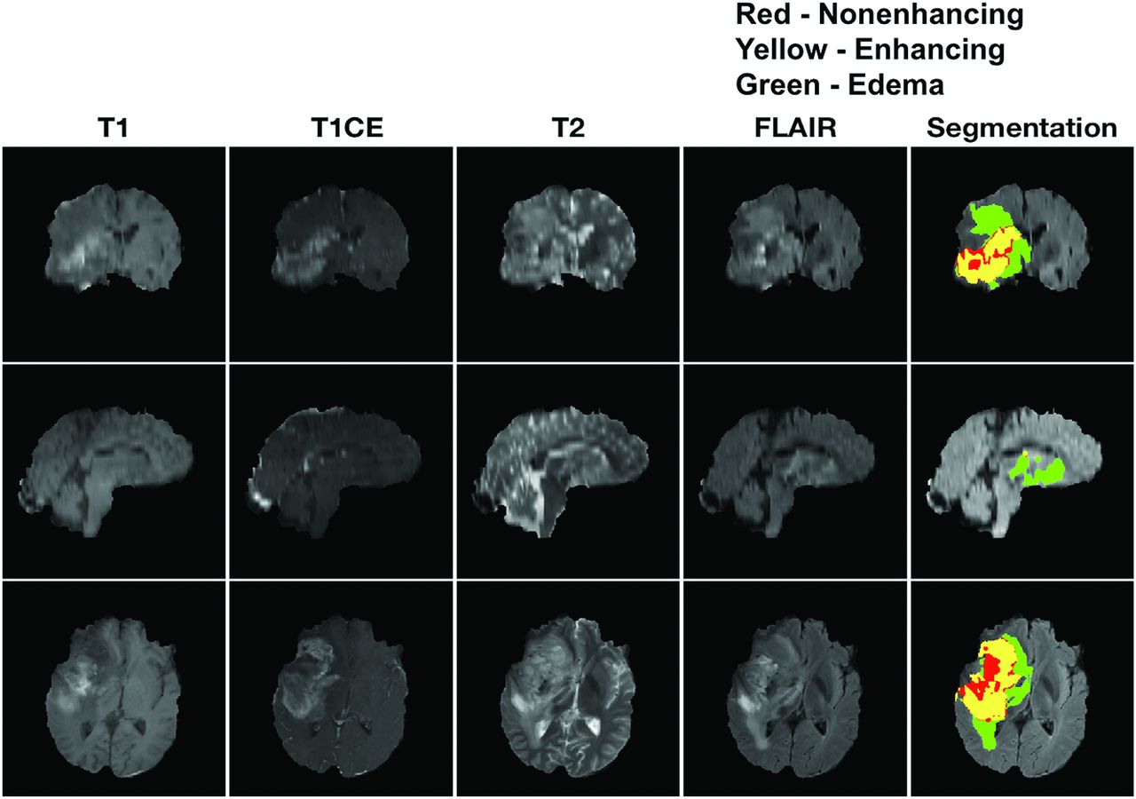
Representative segmentation result from one glioblastoma patient. Top row: Coronal; Middle row: Sagittal; Bottom row: Axial. T1, T1c, T2, and FLAIR are shown in the first 4 column, after being resampled to 1mm, registered, and skull-stripped. The rightmost column corresponds to the segmentation result overlapped on the FLAIR image. Segmentation was performed using cascaded convolutional networks by Wang et al. [21]. In the segmentation image, green corresponds to edema, yellow corresponds to enhancing, and red corresponds to non-enhancing regions.

Confusion matrices of the candidate methods (SVM, RF, GB, and CNN). Top left: SVM; Top right: RF; Bottom left: GB; Bottom right: CNN. Each row corresponds to the true grade and column corresponds to the predicted grade. The main diagonal shown in light grey represents the number of data points that were classified correctly. The off-diagonal numbers are the number of data points that were mis-classified. CNN outperforms the machine learning models by a 23% improvement in accuracy.
Figure 3 contains a comparison of the discussed methods using performance metrics: precision, recall, and F1-score. There is a significant improvement in performance by the proposed CNN method, suggesting that the learned features are valuable in predicting tumor grade.

Comparison of the candidate methods (SVM, RF, GB, and CNN) using three performance metrics. Left: Precision; Middle: Recall; Right: F1-score. The top row corresponds to macro-averaged metrics and the bottom row corresponds to weighted average metrics. Macro-averaging computes the score for each grade and then averages without accounting for class imbalance. On the other hand, weighted average accounts for class imbalance by weighting the metric of each class with the number of samples in that specific class. CNN performs superior to the other models in all of the metrics examined.
Figure 4 contains the activation maps from one representative case for each tumor grade. T1CE images are more strongly activated for high grade (III and IV) compared to low grade (I and II) gliomas. There is a gradual increase in activation of T2 images from grades I to IV. FLAIR images are most strongly activated for grade II. Based on activation maps for the proposed CNN, we infer that T1CE, T2, and FLAIR are the most valuable for identification of grades II to IV respectively. There was no significant activation observed in any of the grade I images. These interpretations were made based on visual inspection of all scans of each grade.

Representative activation maps generated by the proposed CNN (one example per grade). Each row corresponds to a particular grade (I to IV) and each column corresponds to a sequence (T1, T1CE, T2, and FLAIR). Activation by T1CE images was significant for grades III and IV. Activation by FLAIR was most significant for grade II. There was a gradual increase in activation based on T2 images from grades I to IV. T1CE and FLAIR were the most significant sequences for differentiation of low grade (I and II) and high grade (III and IV) gliomas. FLAIR, T1CE, and T2 images produced the strongest activation for grades II, III, and IV respectively.
Figure 5 contains the sequence significance and tumor component significance determined by using the GB algorithm. Among the sequences considered for grading, T1CE and FLAIR were most important, followed by T2. Edema was the most significant tumor component for classification, followed by the enhancing and non-enhancing regions.

Sequence and tumor component significance was determined using a gradient boosting algorithm. The results obtained here comply with the findings of CNN. T1CE and FLAIR were most significant, followed by T2. Edema that is seen in FLAIR plays an important role for classification of different grades.
Figure 6 contains the comparison between validation and test data using weighted average precision, recall, and F1-score to test robustness of the proposed CNN. The error bar corresponds to the 95% confidence interval. Validation data was used to determine the hyperparameters of the network and test data was used to evaluate the performance of the proposed CNN with these hyperparameters. We observed that the performances of the proposed method between validation and test data are consistent, indicating robustness of the proposed method.

Weighted average precision, recall, and F1-score for the validation (red) and test (gray) dataset for proposed CNN method. The performances of CNN are consistent in both datasets, indicating robustness of the proposed method.
DISCUSSION
In this study, we used a convolutional network to classify glioma grades, based on pre- and post-contrast-enhanced MR images, and compared performance against 3 established ML methods. We were able to implement the entire preprocessing pipeline from resampling to tumor segmentation automatically. A neuroradiologist was required only to validate the segmentations. We have leveraged convolutional networks to extract learned spatial features and have used these features to improve prediction of glioma grade from multicontrast MR imaging. This is in contrast to most of the previous studies that rely on radiomic features alone.
The ML methods have poor prediction of grade I compared with the proposed CNN. All of the misclassified grade II tumors were predicted as a higher grade by ML methods. Moreover, at least 70% of the misclassified grade II tumors were predicted as grade IV: SVM = 7/10, RF = 9/11, GB = 12/13. The proposed CNN incorrectly classified grade II as grades I and III. A large proportion of misclassified grade III tumors were predicted as grade II: SVM = 7/17, RF = 13/24, GB = 10/15, CNN = 6/6. All of the methods, except SVM, which had a misclassification rate of 28%, performed well in predicting grade IV tumors with a misclassification rate below 10%. Overall, the methods except GB tended to bias predictions toward a lower grade. SVM overclassified 17 and underclassified 27, RF overclassified 18 and underclassified 24, GB overclassified 21 and underclassified 15, and CNN overclassified 1 and underclassified 12. Distinguishing grades II and III is clinically important for treatment planning. For all the methods, a higher percentage of grade III tumors was predicted as grade II than grade II predicted as grade III. Moreover, most of the errors in ML techniques were due to misclassification of lower grade tumors (Fig 2). This may, in part, be due to the inherent class imbalance of the training set.
Essential to the proposed network was the use of drop-out to prevent overfitting and batch normalization, improving the performance of the network through adjusting and scaling the activations. The results presented in Figs 2 and 3 correspond to test data, which were unseen by the model during training and were used to evaluate the final performance of the network. We observed no difference in performance between the validation and test data (Fig 6), suggesting the robustness of the proposed method.
There are several limitations to this study. First, we did not consider molecular information of the tumors. This was a practical limitation because only a small subset of the cases had molecular information on file. This would be a worthwhile extension if this work were to be replicated with a larger dataset. Second, we considered only structural MR imaging data for this work. In the future, we plan to include additional sequences such as diffusion, perfusion, and susceptibility-weighted images, which may improve the model performance. Third, the experiments in this study were performed on 237 patients with 660 scans, all from a single center. This number is large compared with previous glioma-grading studies10 but is small compared with nonmedical domains.12 Substantially larger datasets will enable one to fully harness the potential of deep learning for prediction of glioma grade. Further testing is also required to evaluate the potential of the proposed algorithm in a multicenter setting, to analyze the effect of scanner systems and acquisition settings on the learned features. Fourth, this study did not consider demographic information of the included population (eg, patient age), which may provide additional discriminatory value. Fifth, a unique biopsy was not performed for every MR image. We assumed that the grade from the biopsy applied to all the scans of that particular patient. Sixth, there could be bias in the patient selection due to rejection of data on the basis of automatic skull-stripping and segmentation failures. This warrants further investigation to determine any specific structural characteristics unique to these tumors. It is worth noting that the state-of-the-art skull-stripping and segmentation are improving at a rapid pace, and we expect a failure rate of these preprocessing modules to diminish with time. Seventh, the number of patients with grade I was very small, creating a data imbalance. This is because patients with grade I tumor are less likely to be referred for surgical biopsy for confirmation. This feature makes it difficult to evaluate the performance of grade I detection; however, in clinical practice, grade I neoplasms tend to be monitored with imaging across time to assess change without necessarily requiring surgical resection. Eighth, about 50% of the scans were excluded either due to poor image quality or failures in skull-stripping and segmentation. These problems must be overcome for broad clinical applicability of automated glioma grading.
This study was performed entirely using 2D slices. A natural extension would be to adapt the proposed network architecture to process the entire 3D tumor volume. This change would substantially increase the number of parameters and reduce the dataset size. Overfitting would become a major concern, even with regularization. We believe a 3D solution would require a dramatic increase in the sample size through ≥1 of the following: 1) access to a larger reference dataset, 2) data augmentation, 3) use of combination approaches that feature-extract using a trained network and classify using ML that are robust to small data sizes,26 and 4) adapting a transfer learning approach.18
There is substantial clinical value in accurate prediction of glioma grade. Direct tissue biopsy is inherently associated with a risk to the patient, has the potential for sampling error, and has a substantial cost in resources. Accurate differentiation between low-grade gliomas (grades I and II) and high-grade gliomas (grades III and IV) has important treatment ramifications and is particularly valuable if this can be done noninvasively and accurately. Because these training data are applied to larger datasets, further ability to differentiate the tumor grade may be more apparent. Ultimately, earlier detection of disease grade using this noninvasive method may be safer and more cost efficient and permit a more timely treatment implementation.
With the availability of appropriate training data, the same or a similar technique can be adapted to other classification tasks, such as prediction of genetic mutations in gliomas27 and classifying a glioblastoma as recurrent disease versus pseudoprogression.28
CONCLUSIONS
We have demonstrated the feasibility of deep learning, specifically deep convolutional networks, to learn relevant spatial features from multimodal MR images. The proposed network that incorporated the learned features was compared against traditional ML approaches (SVM, RF, and GB) and was found to be superior on the basis of precision, recall, and the F1 score. Thus, CNN-based approaches are an effective alternative for accurate prediction of glioma grade and may ultimately optimize efficient diagnosis and treatment planning with the goal of improved health care management in patients with gliomas.
Acknowledgments
We thank Anand Joshi for help with the use of BrainSuite software and Andrew Yock for proofreading the manuscript.
Footnotes
We gratefully acknowledge grant support from the National Institutes of Health (award No. R33-CA225400, Principal Investigator: K.S. Nayak).
Disclosures: Krishna S. Nayak—RELATED: Grant: National Institutes of Health.* *Money paid to the institution.
Indicates open access to non-subscribers at www.ajnr.org
References
- Received April 18, 2020.
- Accepted after revision September 2, 2020.
- © 2021 by American Journal of Neuroradiology


Jump to section
Related Articles
Cited By...
- No citing articles found.