
Abstract
SUMMARY: Although clinical head CT images are typically interpreted qualitatively, automated methods applied to routine clinical head CTs enable quantitative assessment of brain volume, brain parenchymal fraction, brain radiodensity, and brain radiomass. These metrics gain clinical meaning when viewed relative to a reference database and expressed as quantile regression values. Quantitative imaging data can aid in objective reporting and in the identification of outliers, with possible diagnostic implications. The comparison to a reference database necessitates standardization of head CT imaging parameters and protocols. Future research is needed to learn the effects of virtual monochromatic imaging on the quantitative characteristics of head CT images.
“… it became apparent that the conventional methods were not making full use of all the information the x-rays could give.”
G. Hounsfield, Nobel Lecture, 19791
CT scans serve a unique and necessary role in clinical medicine with approximately 82 million CT scans performed in the United States in 2018, and 11.5 million of those being head CTs.2,3 Despite these numbers, the radiation exposure from CT largely precludes prospective human subjects research. In addition, low soft tissue contrast has resulted in relatively little published clinical research in head CT imaging relative to MR imaging. In the clinical setting, CT is used to diagnose gross structural pathology, to be followed by MR imaging as clinically indicated. Where the signal intensity of MR imaging is largely uncalibrated, the image intensity of CT is a scaled and calibrated metric that reflects the radiodensity of the material imaged and offers a quantitative tissue measure, which is not assessed by MR imaging. In this review, we discuss current methods and applications of quantitative analysis of head CT imaging.
Methods of Analysis
Volumetric analysis of brain CT imaging entails removal of nonbrain tissue from the head imaging series, an image-processing step termed “brain extraction” or “skull stripping.” Brain extraction is often performed in postprocessing of brain MR images and has been less applied to CT imaging. Several author groups have found that the MR imaging postprocessing software FSL (http://fsl.fmrib.ox.ac.uk/fsl/fslwiki/FSL)4 can be used to process head CT imaging.5,6 By means of FSL, the skull can be subtracted from head CT images by thresholding, and the residual nonbrain tissue can be removed using the FSL Brain Extraction Tool (http://fsl.fmrib.ox.ac.uk/fsl/fslwiki/BET). The CSF space can be subtracted to permit the calculation of the ratio of the brain volume to intracranial volume, to yield the brain parenchymal fraction.7,8
Volumetrics
Digital images are acquired as signal intensities with voxel coordinates. The routine CT brain protocol at our institution results in voxels that are 0.5 × 0.5 mm and are typically displayed and stored at 5-mm section thickness, with the consequence that the spatial resolution is very high in-plane (“x” and “y” dimension on an axial section) but low in the “z” dimension. After brain extraction, the volume of the brain parenchyma can be obtained by a simple voxel count, which is easily performed with FSL. The average adult brain size is approximately 1200 cm3, or on the order of 1,000,000 voxels.
Changes in brain volume as a function of age have been a popular topic of imaging literature, largely investigated with MR imaging of healthy volunteers.9⇓⇓-12 Abnormalities of total brain volume have been associated with congenital and acquired pathology. In the pediatric population, congenital conditions are associated with macrocephaly and microcephaly, with accompanying abnormalities of brain volume. Among adults, abnormalities of global brain volume have been described in multiple sclerosis,8 amyotrophic lateral sclerosis,13 and Alzheimer disease and age-related dementia.14,15 Head CT has been used for the investigation of brain volume measures in Alzheimer disease and age-related dementias well before the advent of MR imaging. Early studies focused on CT brain volumetrics as derived or inferred from linear measurements, such as sulcal width or ventricular volume.16 Recent advances in computer software enable automated, statistical modeling of digital methods of analysis of head CT images. Quantitative assessment of brain volume could aid in the characterization of pathology associated with global brain volume loss.
The Brain Parenchymal Fraction
Where brain volume varies widely among healthy individuals, the ratio of the brain volume to the intracranial volume, or brain parenchymal fraction, reduces the intrasubject variability.8,17 Accurate estimation of the brain parenchymal fraction requires estimation of the intracranial volume and the brain volume, the latter measure achieved by segmenting the CSF from the brain parenchyma. The brain parenchymal fraction increases sensitivity for correlation with pathology, is decreased in multiple sclerosis, and has been used to distinguish different phenotypes in amyotrophic lateral sclerosis.8,13 The brain parenchymal fraction shows consistent decline with age after the second decade, with decreased variance relative to the brain volume measure (Fig 1 and Cauley et al7,18).

Change in brain parenchymal fraction through the life span, men (filled) and women (unfilled). This figure summarizes the findings further detailed in Cauley et al.7
Radiodensity
During CT imaging, the radiodensity of each voxel is recorded as the signal intensity and is scaled and calibrated in terms of the Hounsfield unit (HU), a scale that defines “zero” for distilled water and −1000 for air.1 More precisely, the HU scale “is a linear transformation of the original linear attenuation coefficient measurement into one in which the radiodensity of distilled water at standard pressure and temperature is defined as 0 HU, while the radiodensity of air at [standard pressure and temperature] is defined as −1000 HU.” For materials of higher attenuation, the HU for bone is on the order of 1000–2000 HU and for metal, > 3000 HU.19
In a voxel with average linear attenuation coefficient μ, the corresponding HU value is therefore given by
 where μwater and μair are the linear attenuation coefficients of water and air, respectively. This definition is true for CT scanners that are calibrated with reference to water.
Although the radiodensity value is only infrequently used in routine image interpretation, the accuracy of the radiodensity determines the image quality, and it is monitored and calibrated as part of the American College of Radiology quality control program (ACR.org). In our studies using standard clinical CT scanners, the Hounsfield units of water and of an attenuation phantom are recorded daily and drift or trending were rarely observed. In a typical month, the HU of water or the tissue attenuation plug is found to vary by less than 1 HU.
Radiodensity assessment of the brain enables objective, quantitative assessment of findings which are typically described in qualitative terms. Such quantitation enables the detection of subtle changes that might otherwise be overlooked. Radiodensity measures of specific pathologies, such as hemorrhage or cerebral edema after infarct, have been investigated with claims of prognostic implication.20,21 There are few reports on the radiodensity of nonfocal or global parenchymal pathology.22 Using automated, digital methods, a decline in global radiodensity of the brain as a function of aging has been reported.7 Using digital methods a higher global brain radiodensity was found in multiple sclerosis.23 Others report a globally decreased brain radiodensity associated with elevated intracranial pressure.24 Global radiodensity values in the context of quantile regression, as described below, may aid in the identification and characterization of conditions involving abnormalities of global brain radiodensity.
Radiomass
Tissue volume is arguably the most common metric assessed from imaging. The corresponding postmortem metric is brain tissue weight or mass. The weight might be estimated from the measured volume, provided that the specific gravity (grams/milliliter) of brain tissue is constant.11 This would not appear to be the case, however, as the radiodensity increases in early life25 and decreases with age.7 An alternative weight estimation for CT imaging is the product of the volume and the radiodensity, or the “radiomass.” Although the radiomass has the cryptic units of HU ×cm3 and has been little explored in the literature, the measure may have clinical meaning. Study results vary, but whereas the brain volume declines approximately 11% throughout the adult life span,26 the brain weight declines 20%–22%. Compared with postmortem literature, the measured relative decline in radiomass as a function of age is highly correlated with direct measures of brain weight (unpublished data). Disease states may also show changes in brain radiomass, though this has not been investigated. In multiple sclerosis, for example, brain volume and radiodensity are both affected by the disease.8,23 Future studies will be needed to investigate correlations between abnormalities of radiomass and various global brain pathologies.
Gray and White Matter Segmentation
Imaging research is facilitated by segmentation of tissue types and anatomic regions. Where tissue class segmentation is relatively straightforward for MR imaging, low image contrast poses a challenge for gray-white matter segmentation of CT images. When displayed as a voxel histogram, MR imaging is of sufficient image contrast that gray and white matter are represented as separate peaks of a bimodal distribution of signal intensity (Fig 2).27 For clinical brain CT images, however, the signal intensity histogram of the brain is unimodal, without separation between gray and white matter peaks (Fig 2 and Cauley et al6). Tissue class segmentation of head CT images requires a more sophisticated methodology than a simple radiodensity cutoff.

Segmentation of CT images can be direct, based on the signal intensities of individual voxels6 or based on image masking using an MR imaging template.28 Newer techniques propose machine learning algorithms for CT image segmentation.29 Although MR imaging represents a current “gold standard” for segmentation, gray and white matter segmentation of MR images can vary with segmentation technique.30 A given voxel may include a mix of tissue classes, and accurate segmentation entails subvoxel segmentation. Direct segmentation, as described using software such as FSL, has both binary and partial volume options. A comparison of the outputs of binary and partial volume segmentation is shown in Fig 2. Gray and white matter volumes derived from brain CT segmentation are likely to differ from MR imaging results, though a direct comparison of segmentations from the different modalities has yet to be conducted.
Segmentation of brain CT images enables measurements of gray and white matter radiodensity, which may have clinical implications. In cases of global anoxic injury seen in cardiac arrest, for example, the gray matter radiodensity decreases and consequently the ratio between gray and white matter densities is decreased.31 Automated segmentation can facilitate this calculation.32 It has recently been suggested that such measures may prove useful in forensic medicine to aid in determining the cause or time of death.33
The Normative Clinical Database. Quantile Regression.
A patient's medical data become meaningful only through comparison to reference values. Existing reference imaging databases of human brain data largely comprise MR imaging studies with relatively small numbers of healthy volunteers. As CT scans entail a radiation exposure, the recruitment of healthy volunteers into a CT study for this purpose would be difficult to justify. However, in the clinical setting, the threshold for CT imaging is very low, and the PACS includes large numbers of studies with essentially normal findings. Radiographic studies with normal findings can be narrowed to studies of patients without significant medical history or without systemic disease. In this way, large databases can be subject to statistical analysis to identify normative parameters.
A criticism of a database generated from the clinical archive is that because patients are always scanned for a reason, no study within the database can be presumed to have truly normal findings, and therefore, such a database cannot serve as a reference. This reasoning should be questioned. First, many studies within the archive are performed for nonspecific symptoms or for minor trauma without traumatic finding and have essentially normal findings. As the database increases in size, the mean values will approach normalcy. Second, our goal is not to identify the healthy patients, but to identify the patients with abnormal findings. In the clinical setting, a patient's condition is judged as more or less urgent. In this sense, the metrics of a given study need not be identified as healthy or unhealthy, but rather “at the 97th percentile” or “at the 23rd percentile” (of brain volume for age and sex, for example), as is often done for other types of clinical data. This can be achieved through quantile regression (Fig 3). This is the reasoning by which the diagnosis is made for microcephaly (head circumference > 2 SD below the mean for sex and age)34 or macrocephaly (head circumference of > 2 SD above the mean for age and sex).35 Databases could be continuously expanded as studies meeting criteria for “negative” or healthy are added. Finally, the PACS archive offers a huge database of both sexes across the life span. Such a cohort would be difficult to obtain through the recruitment of healthy volunteers. As a prospective study is not likely to happen, the PACS database is the only information available for the generation of a reference database for CT images.
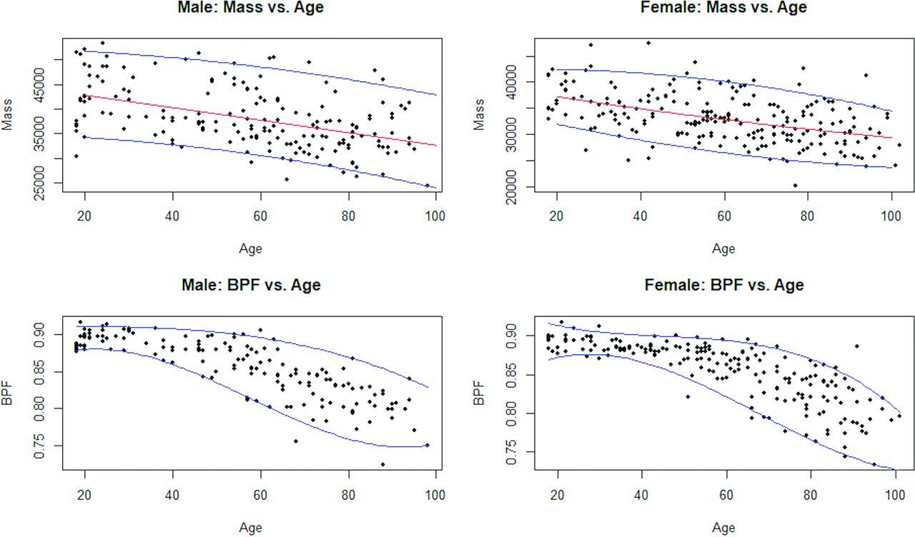
Quantile regression of adult brain parenchymal fraction (men, left and women, right) as a function of age. Quantile regression of adult brain mass (men, left and women, right) as a function of age.
Caveats and Current Limitations of Quantitative CT
Manipulation of CT Images.
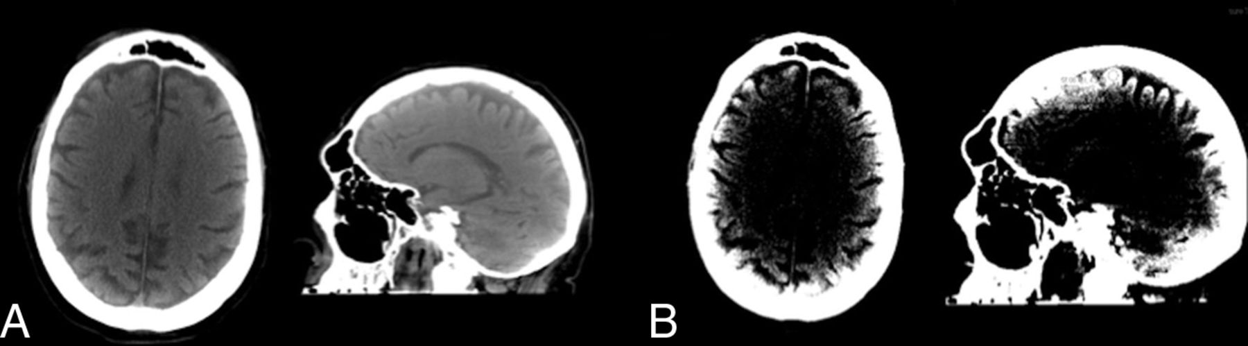
Popular MR image processing techniques, such as image registration (warping), are not as easily applied to CT imaging due to typically highly anisotropic voxel geometry and changes in the partial volume calculation. Changing the positioning or angulation of the CT brain image after acquisition can alter volume measurement (Fig 4A, -B). Registering CT images to a target image can alter the CT image histogram (Fig 4A, -C) and erode the image integrity. Warping the images while maintaining the integrity of the signal intensity may be a complex task.36 As an alternative, mask or standard images can be registered to the CT scan enabling gross registration of standard atlas images.

The effects of image rotation on radiodensity histogram and volumetrics of brain CT images. A, Original image. Volume calculated 1565 mL. B, Image rotated 15° to the right. Volume calculated 1602 mL. C, Rotated image registered to standard brain MR imaging template in FSL to restore image to nonrotated orientation. Volume calculated 2022 mL.
Beam-Hardening by the Skull.
Since the initial development of head CT imaging, it has been noted that the high attenuation of the skull creates a significant beam-hardening artifact, which greatly limits image quality.37,38 This artifact is greater for thicker skulls, and can impact image interpretation.6,39 Modifications in machine design have enabled prehardening of the beam, reducing the effects of beam-hardening on the images;40,41 however, the effects can still be seen on many current acquisitions (Fig 5 and Cauley et al6). Radiologists tend to associate beam-hardening with streak artifacts, which are caused by focal skull thickening or by sharp attenuation transitions between air and skull, as in the paranasal sinuses. Beam-hardening is a far more universal phenomenon in head imaging, as the skull filters all x-rays that pass through it and increases the mean beam energy reaching the brain (increasing the kilovolt peak). This in turn results in a decrease in the measured HU as the brain tissue has less stopping power for higher energy x-rays. This broadly affects the measured HU of brain tissue and draws attention to the fact that HU measures are not absolute. The effects of beam-hardening are reduced by a monochromatic x-ray source.42
Beam-hardening by the skull is seen in routine clinical head CT. These images were acquired on 11/14/2018 from a standard hospital GE Healthcare scanner for acute trauma. For the image pair on the left the default display window settings were used (window width/window length 125/40). For the image pair on the right (same case), the display window settings were window width/window length 17/42. This persistent beam-hardening artifact can impact the interpretation of cortical lesions and is particularly important when performing quantitative, digital analysis.
In MR imaging, field inhomogeneities can give rise to image intensity inhomogeneities, which can undermine image quality and preclude accurate image processing, such as registration and segmentation (Fig 6). Postprocessing software has been developed for image intensity inhomogeneity correction of MR images and has been used to facilitate automated segmentation algorithms.43,44 We found that ictal-interictal continuum algorithms developed for use in MR imaging can identify the global signal inhomogeneity of head CT imaging caused by the beam-hardening of the skull (Fig 7). Examples include the ITK N4BiasFieldCorrection Filter (https://simpleitk.readthedocs.io/en/master/link_N4BiasFieldCorrection_docs.html), as well as the correction factor that is engineered into the FSL Automated Segmentation Tool (http://fsl.fmrib.ox.ac.uk/fsl/fslwiki/FAST), which facilitates CT segmentation in much the same way as it facilitates MR imaging segmentation.6 Because beam-hardening by the skull is dependent upon the thickness of the skull through which the beam passes, head positioning in the scanner can influence the beam-hardening, and therefore, influence the measured radiodensity. The head position can be “corrected” as a postprocessing step at the console, but the beam-hardening effects will persist in the image. For this reason, the use of a head holder and attention to patient positioning are advised for quantitative CT.

Image inhomogeneity seen on routine MR images of the brain, with image intensity inhomogeneity–corrected image on the right. Reproduced with permission from Vovk et al.44
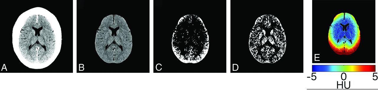
FSL “Bias field reduction” corrects for the attenuation and scatter artifacts seen on routine clinical head CT images. Subject with a thick skull and normal head CT (A). Brain-extracted image (B). Segmented GM images with “bias field correction” “turned off” (C), and with bias field “on” at default settings (D). The magnitude of the correction in HU, color-scaled as per the color bar at the bottom (E). Reproduced with permission from Cauley et al.6
Machine Calibration.
There is calibration drift within individual scanners, as well as small differences in measured radiodensity between scanners from the same manufacturer running the same protocol, though data trends appear consistent.25
Greater differences might be expected from machines from different vendors or using different protocols. Until more rigorous standards are established, statistical methods of normalization may be necessary for the adaptation of a universal database to a particular setting.
The Role of Quantitative Assessment in Clinical Medicine.
As with most quantitative diagnostic tools, quantitative CT must be interpreted in a clinical context. There has been considerable investigation into the value of the gray and white attenuation ratio in assessing the degree of hypoxic-ischemic injury in the setting of cardiac arrest.31,32,45⇓-47 Brain volume, radiodensity, or radiomass identified as statistically higher or lower than a comparative peer group may have normal findings, or it may raise suspicion for a particular pathology, or serve to support an existing suspicion of a particular pathology. In cases of known disease, quantitative CT may be used to monitor disease status.
Future Directions
Machine Calibration.
American College of Radiology guidelines for the calibration of CT scanners are sufficient for the maintenance of image quality, but may not be optimal for quantitative imaging. At our institution, daily machine calibrations are recorded and note little (typically less than 1 HU) variation; however, calibration is performed in the same way and at the same time every day. Drift of HU values throughout the day or after high usage is not typically evaluated. Calibration values are recorded but not rigorously reset to zero when small drifts are observed. The range of radiodensities of brain tissue is relatively narrow, with the bulk of the brain tissue radiodensities falling between 15 and 40 HU, and small differences in mean radiodensity may represent significant tissue differences, as a 3-HU difference in mean brain tissue radiodensity was found between control subjects and patients with multiple sclerosis. Higher standards for machine calibration would not be difficult to achieve. The measured HU could be rezeroed daily, rather than be permitted to drift between accepted values. A water standard could be included with each imaging study, perhaps as part of the imaging apparatus, such that the image intensity could be referenced to an internal zero standard.
Anatomic Segmentation.
A large body of research in MR imaging has focused on volumetric changes that occur in specific anatomic brain regions.48⇓⇓-51 The relatively low image contrast of CT has precluded this type of analysis of head CT images. Although it is possible to localize brain regions using MR imaging-based atlas images to mask CT images, further research in this area is needed before reliable regional measures can be derived from head CT images. Although still in its early stages, machine learning may prove useful in this regard.52 If gray and white matter have discrete radiodensities, the radiodensity of a given lobe or anatomic segment of brain would be expected to largely reflect the percentages of gray and white matter in a particular substructure, though this idea has yet to be verified empirically.
Dual Source CT.
As discussed above, the beam-hardening artifact from the skull has long posed a problem for head CT imaging. Beam-hardening by the skull is the result of filtering of lower energies of the x-ray energy spectrum. Dual Source CT (Siemens) has been advocated for metal artifact reduction53 and dual source virtual monochromatic imaging has the potential to reduce beam-hardening caused by the skull,54 though this too has yet to be fully investigated. Reduction in beam-hardening could result in more reliable quantitative imaging, with the caveat that changes in image acquisition may confound comparison with previously acquired images using conventional methods. Similarly, standardization of protocols (kilovolt peak and milliampere settings, pulse width [milliseconds], helical versus axial imaging) should broaden the application of quantitative imaging.
CONCLUSIONS
Godfrey Hounsfield noted that the quantitative capability of CT is one of its major advantages over 2D x-ray,1 yet the quantitative capabilities of clinical head CT remain largely unexplored. Automated methods together with a clinical database and quantile regression techniques could enable quantitative assessment of head CT parameters to augment qualitative image interpretation.
Footnotes
This work was supported by a Geisinger clinical research fund to K.A.C. and S.W.F., SRC-L-58.
References
- Received February 8, 2021.
- Accepted after revision February 19, 2021.
- © 2021 by American Journal of Neuroradiology


Jump to section
Related Articles
Cited By...
- No citing articles found.